Birth Control vs Inflammation over menses

Study Description

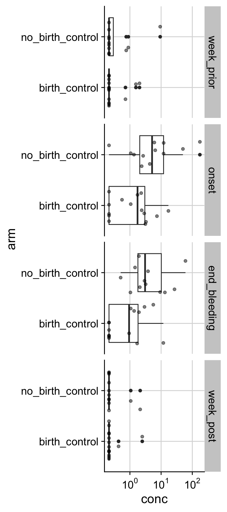
This is an observational study to evaluate the relationship between birth control and vaginal inflammation In response to menstruation. Absolute abundance of bacteria was measured by 3 qPCR assays (for total Bacteria, L. crispatus, L. iners). Cytokine levels (in copies/ml of vaginal fluid) were also measured by Luminex. We also looked at the number and type of immune cells in the vagina using Flow Cytometry. Data was collected at four timepoints; before, at the start, the end, and after menstruation.

Primary Aim

To investigate whether taking birth control is associated with vaginal inflammation throughout the menstrual cycle.

Data processing

library(tidyverse)
library(tableone)
library(cowplot) # load for the theme
theme_set(theme_cowplot(16) + background_grid()) # set cowplot theme

sample_map <- read_csv("data/00_sample_ids_period.csv")
metadata <- read_csv("data/01_participant_metadata_period.csv")
luminex <- read_csv("data/02_luminex_period.csv")
flow_cytometry <- read_csv("data/03_flow_cytometry_period.csv")

Merging the dataset

merged_dataset <- 
  sample_map %>%
  left_join(metadata) %>%
  left_join(luminex) %>%
  left_join(flow_cytometry) %>%
  mutate(cd4_ratio = cd4_t_cells / cd3_positive )  %>%
  mutate(time_point = fct_relevel(time_point,"week_prior","onset","end_bleeding", "week_post"))

Let’s create table one

processed_for_tableone <- merged_dataset %>%
  select(-limits, -sample_id) %>%
  pivot_wider(names_from = cytokine, values_from = conc) %>% # move cytokine to wide
  filter(time_point == "week_prior") # we just want baseline characteristics for table 1

CreateTableOne(
  data = processed_for_tableone,
  vars = c("age", "pcos_status", "period_product", "cd4_ratio", "IL-1a", "IL-1b", "IP-10", "MIG", "TNF-a" ),
  factorVars = c("pcos_status","period_product" ),
  strata = "arm",
  test = FALSE
) %>%
  print(
    nonnormal = c("cd4_ratio", "IL-1a", "IL-1b", "IP-10", "MIG", "TNF-a"),
    
  )

                          Stratified by arm
                           birth_control          no_birth_control      
  n                            15                     12                
  age (mean (SD))           30.80 (2.54)           32.08 (3.20)         
  pcos_status = pcos (%)        6 (40.0)               8 (66.7)         
  period_product (%)                                                    
     menstrual_cup              2 (13.3)               2 (16.7)         
     pad                        3 (20.0)               1 ( 8.3)         
     tampon                    10 (66.7)               9 (75.0)         
  cd4_ratio (median [IQR])   0.51 [0.47, 0.52]      0.45 [0.38, 0.52]   
  IL-1a (median [IQR])      25.65 [11.97, 44.53]   40.94 [11.66, 87.95] 
  IL-1b (median [IQR])       0.24 [0.24, 2.04]      0.24 [0.24, 4.91]   
  IP-10 (median [IQR])      11.80 [6.71, 45.20]    16.95 [6.38, 84.45]  
  MIG (median [IQR])       151.24 [47.17, 301.19] 129.69 [18.63, 365.59]

Arm cytokines

merged_dataset %>%
  filter(cytokine == "TNFa") %>%
  ggplot(aes(x=conc, y=arm)) +
  geom_boxplot() +
  geom_jitter(alpha = 0.5) +
  scale_x_log10(labels=scales::label_log()) +
  facet_grid(rows=vars(time_point), scales="free")

merged_dataset %>%
  ggplot(aes(x=conc, y=arm)) +
  geom_boxplot() +
  geom_jitter(alpha = 0.5) +
  scale_x_log10(labels=scales::label_log()) +
  facet_grid(rows=vars(time_point), cols=vars(cytokine), scales="free")

Time series visualization

merged_dataset %>%
  ggplot(aes(y=conc, x=time_point)) +
  geom_boxplot() +
  geom_point(alpha = 0.5) +
  geom_line(alpha=0.5, aes(color=arm, group=pid)) +
  scale_y_log10(labels=scales::label_log()) +
  facet_grid(rows=vars(cytokine), scales="free")

Cytokines vs pcos

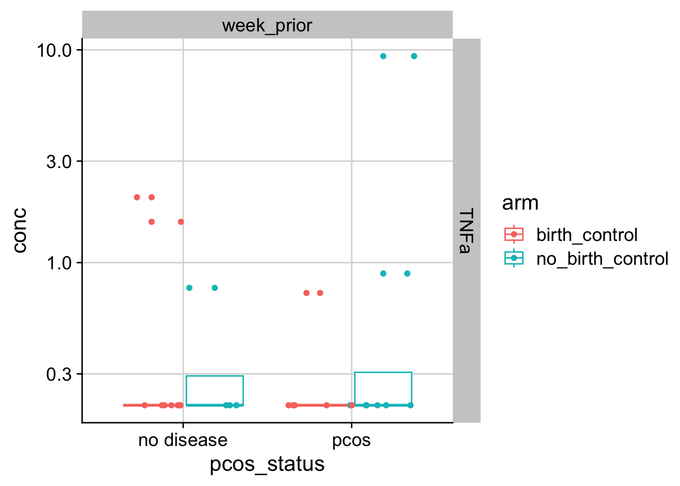
How does PCOS associate with inflammation over menstruation? First, let’s look at one of the cytokines at one of the timepoints.

merged_dataset %>%
  filter(time_point == "week_prior", cytokine == "TNFa") %>%
  ggplot(aes(x = pcos_status, y=conc, color = arm)) +
  geom_boxplot() +
  geom_point(position = position_jitterdodge()) +
  scale_y_log10() +
  facet_grid(cols=vars(time_point), rows=vars(cytokine), scales="free_y")

Now, let’s look at all the cytokines together with all time points.

merged_dataset %>%
  ggplot(aes(x = pcos_status, y=conc, color = arm)) +
  geom_boxplot() +
  geom_point(position = position_jitterdodge()) +
  scale_y_log10() +
  facet_grid(cols=vars(time_point), rows=vars(cytokine), scales="free_y")

Cytokines vs flow

Are there any relationships between cytokines and cd4 ratio?

merged_dataset %>%
  ggplot(aes(x=conc, y=cd4_ratio, color=arm, )) +
  geom_point() +
  scale_x_log10(labels=scales::label_log()) +
  facet_wrap(~cytokine)