R refresher (Brief review of Workshop I)
remixed from Claus O. Wilke’s SDS375 course and Andrew P. Bray’s quarto workshop
Stickies
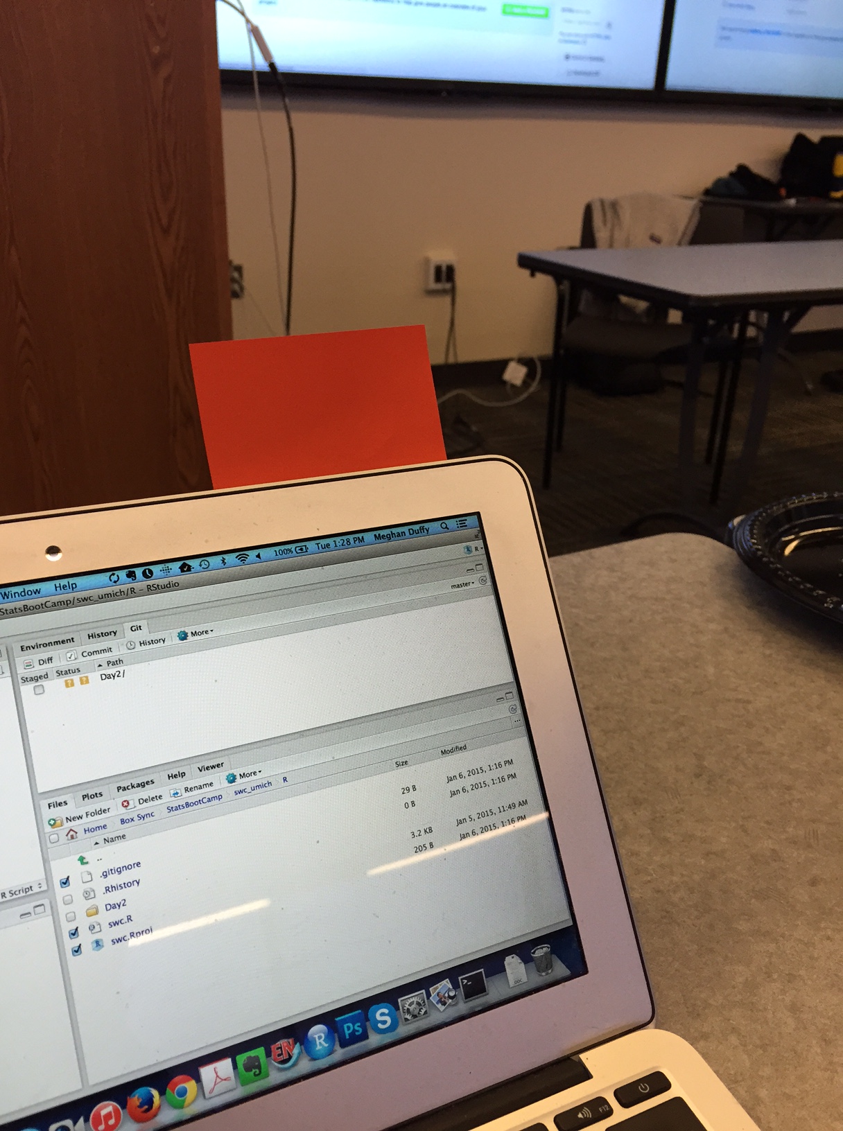
During an activity, place a yellow sticky on your laptop if you’re good to go and a pink sticky if you want help.
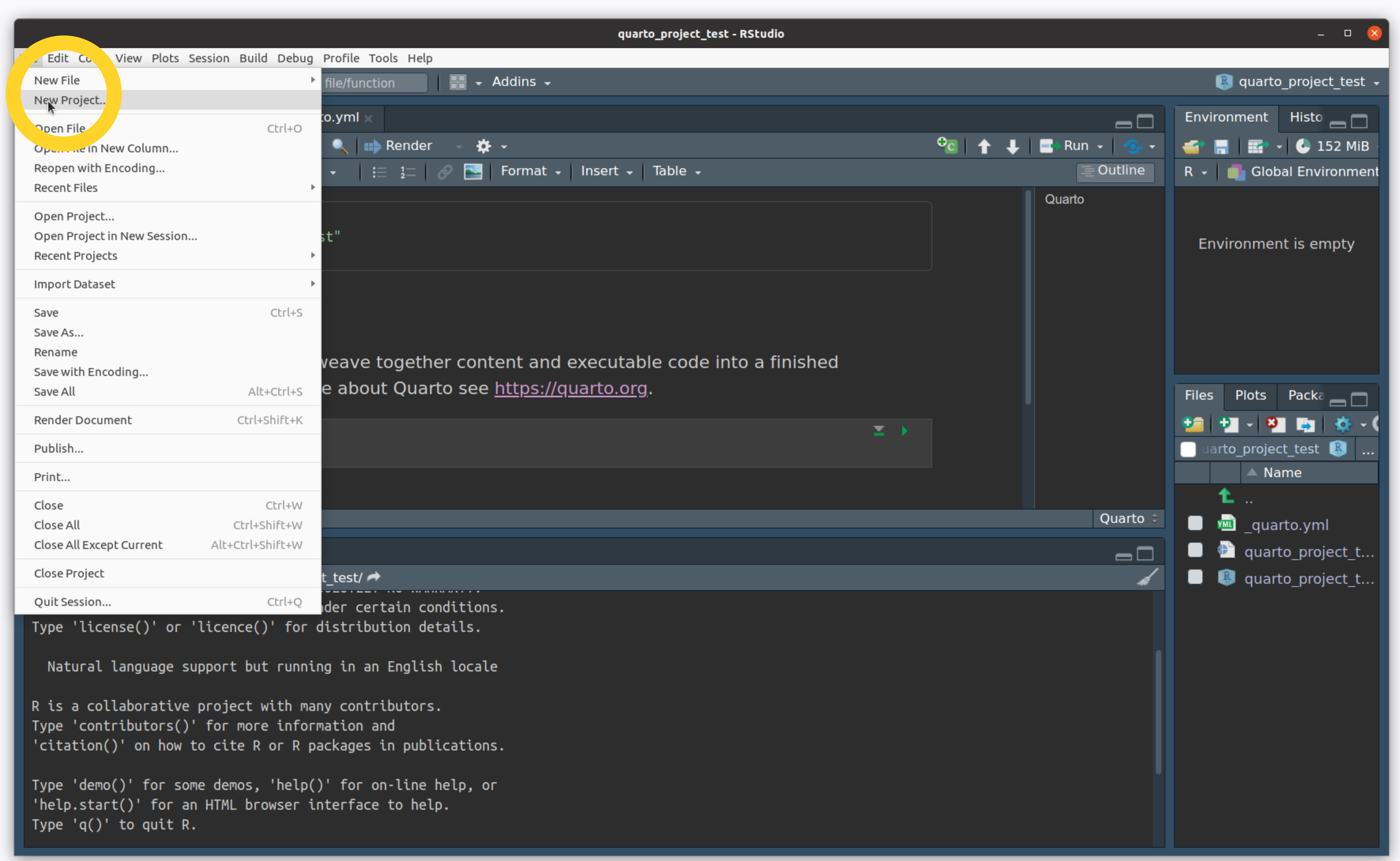
Create an R Project
- File -> New Project…
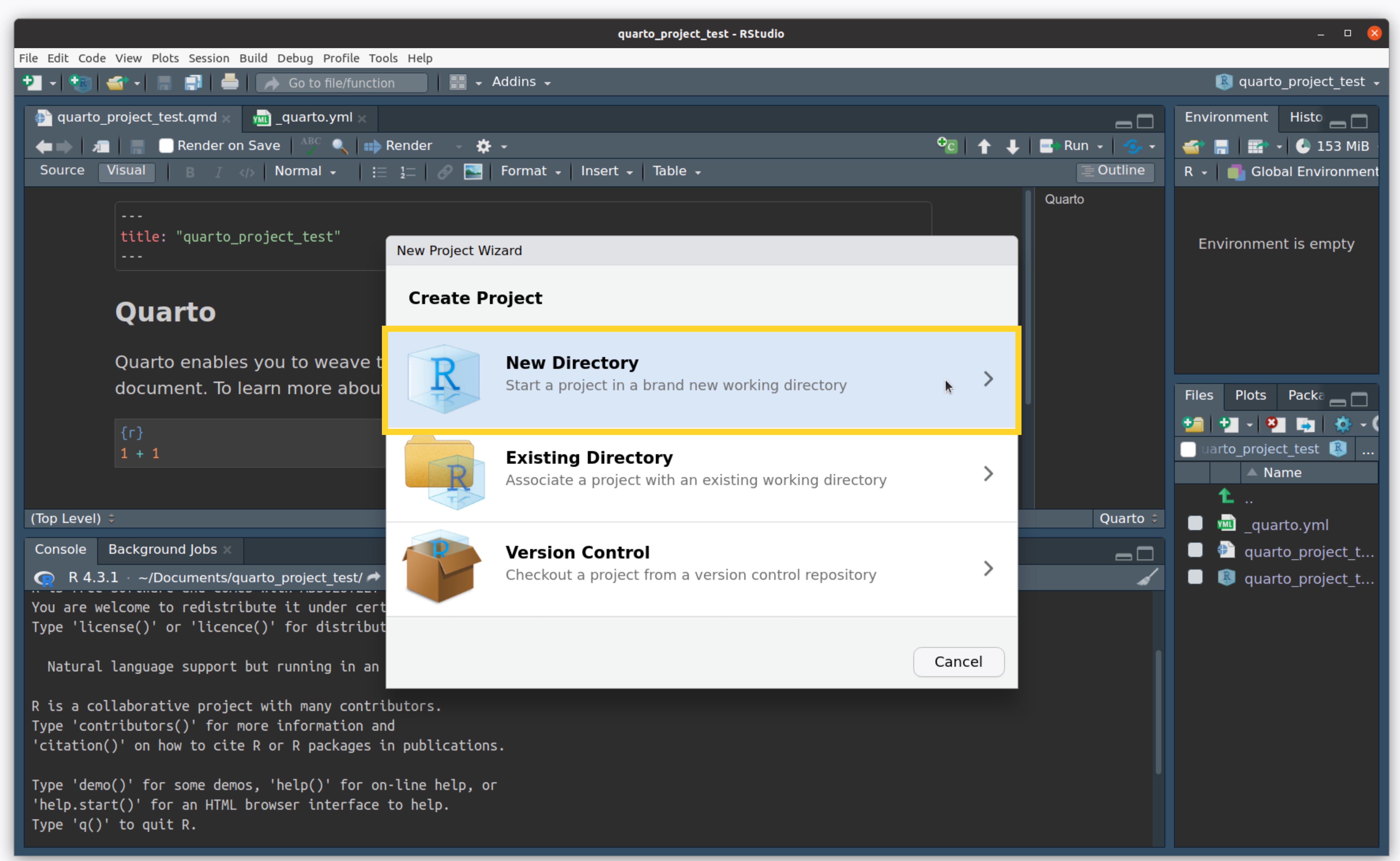
Create an R Project
- Click on New Directory
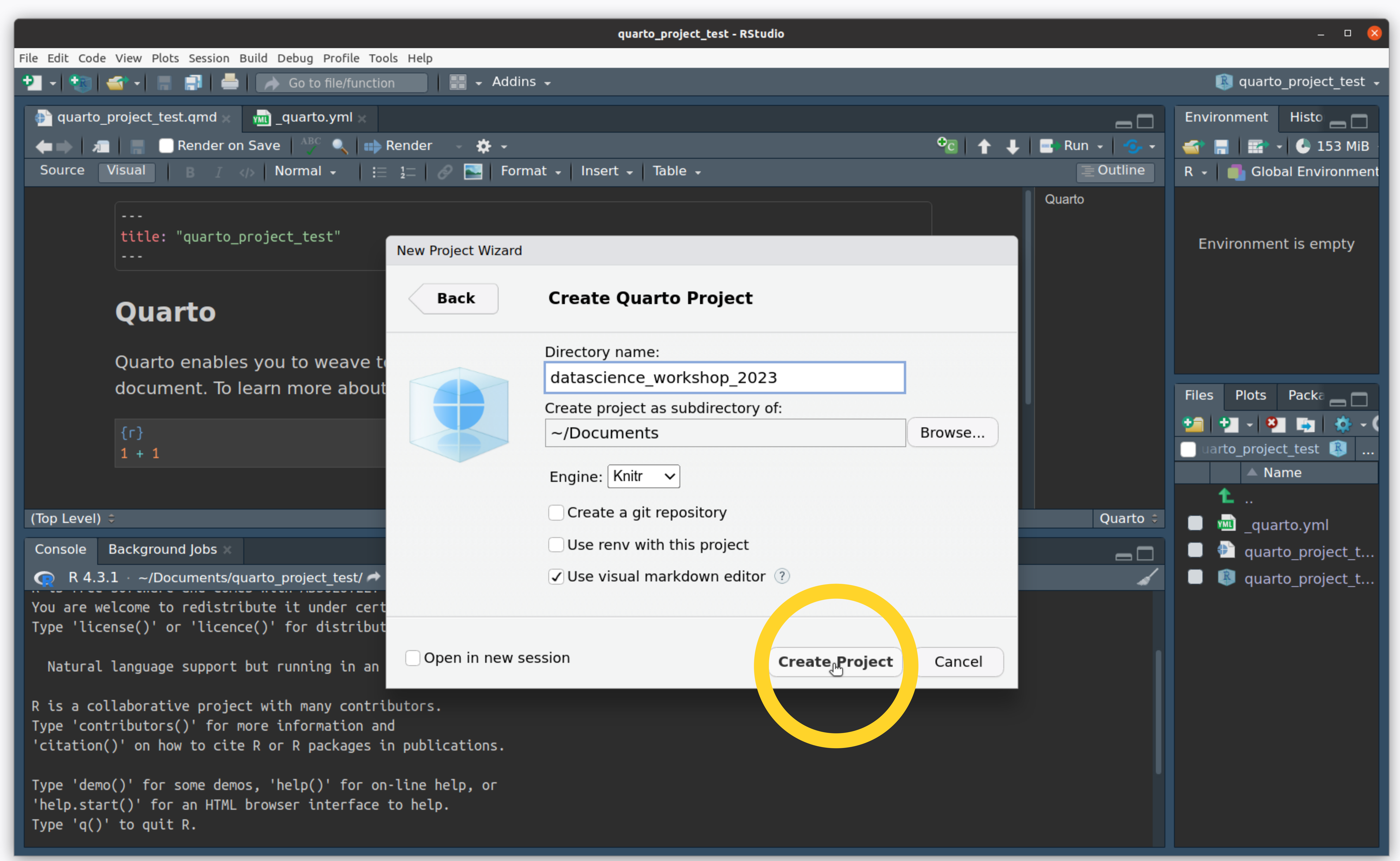
Create an R Project
- Navigate to the
workshop_2folder name your directory and click “Create Project”
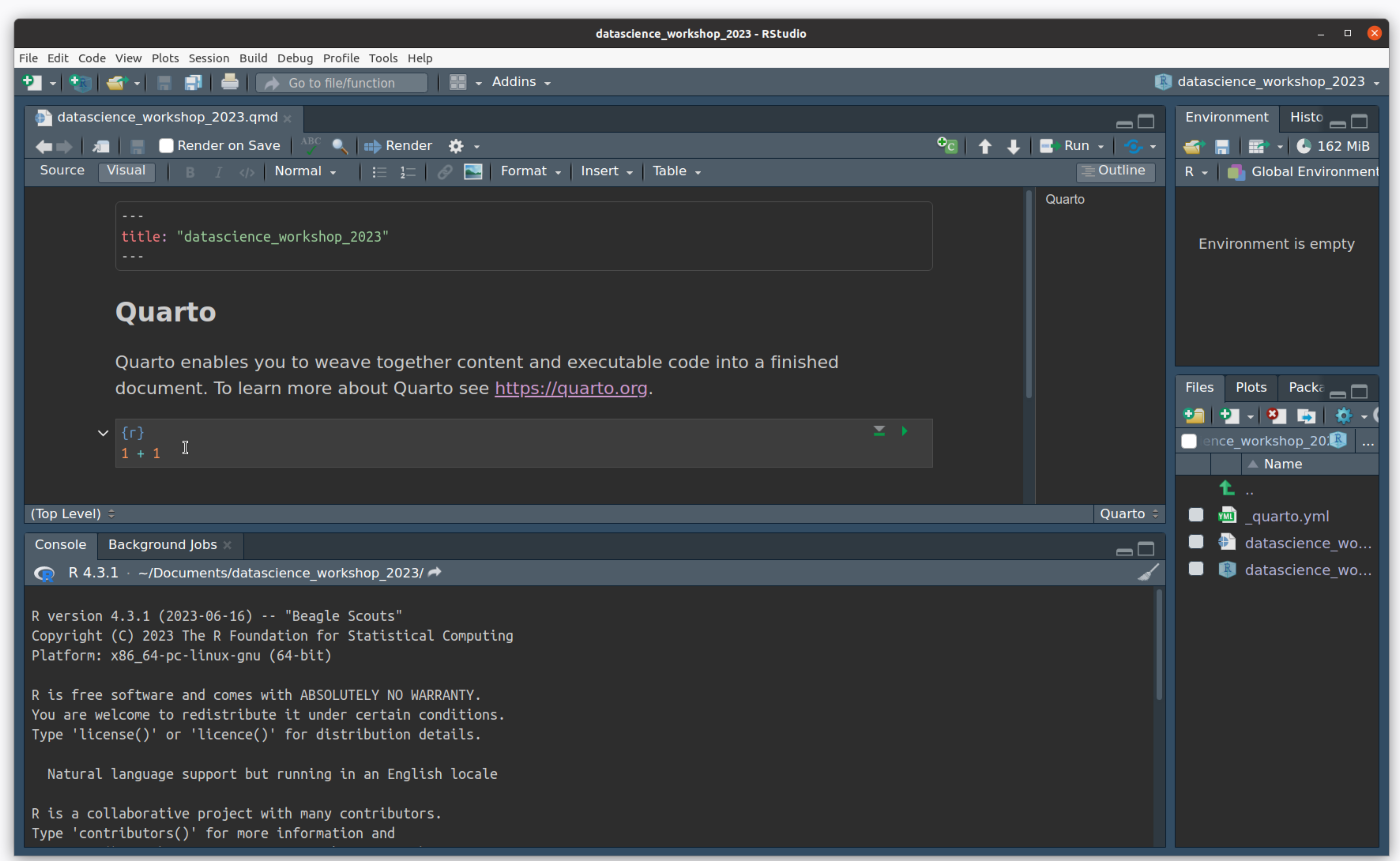
Create an R Project
- You made a project! This creates a file for you with the
.qmdextension
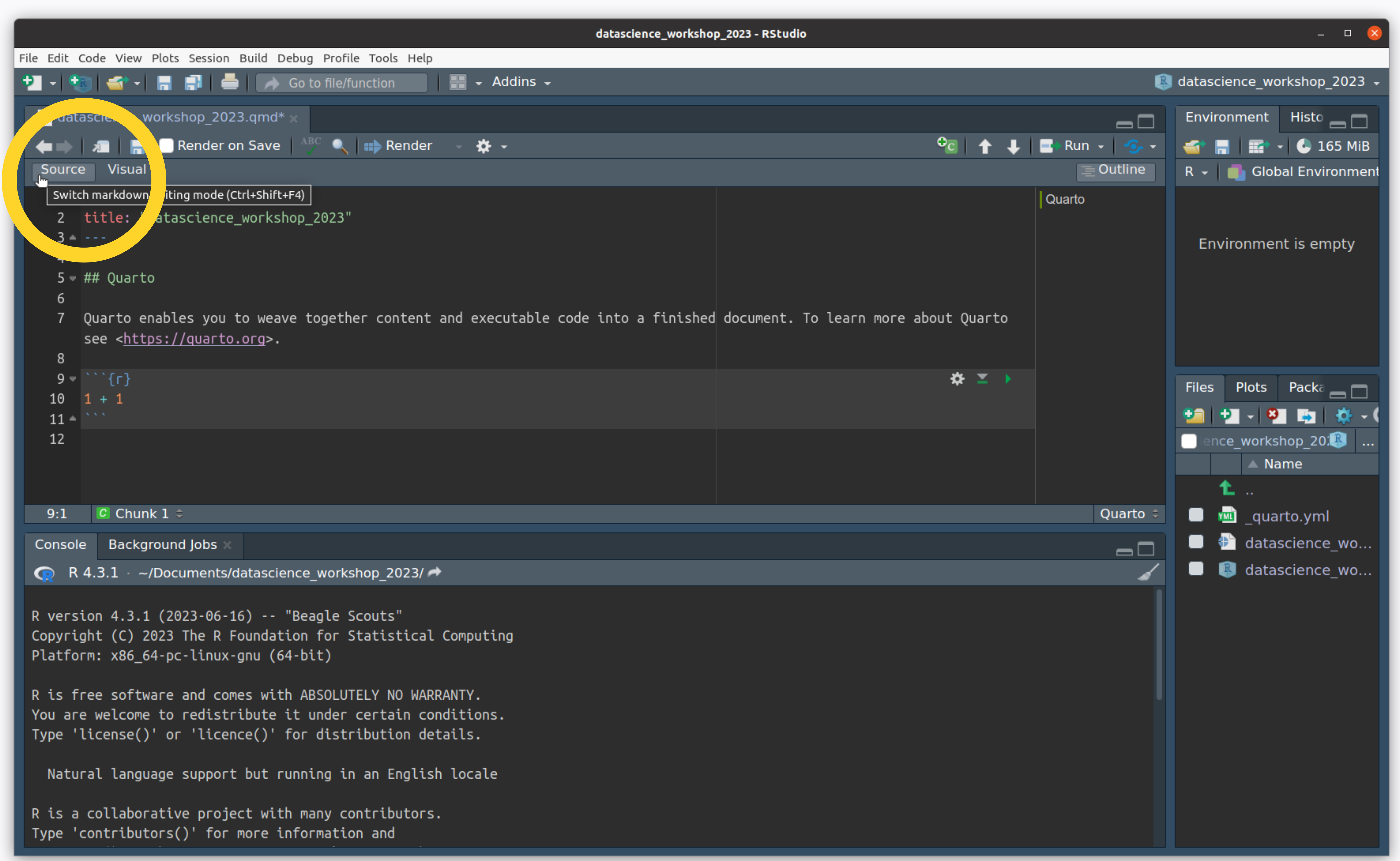
Create an R Project
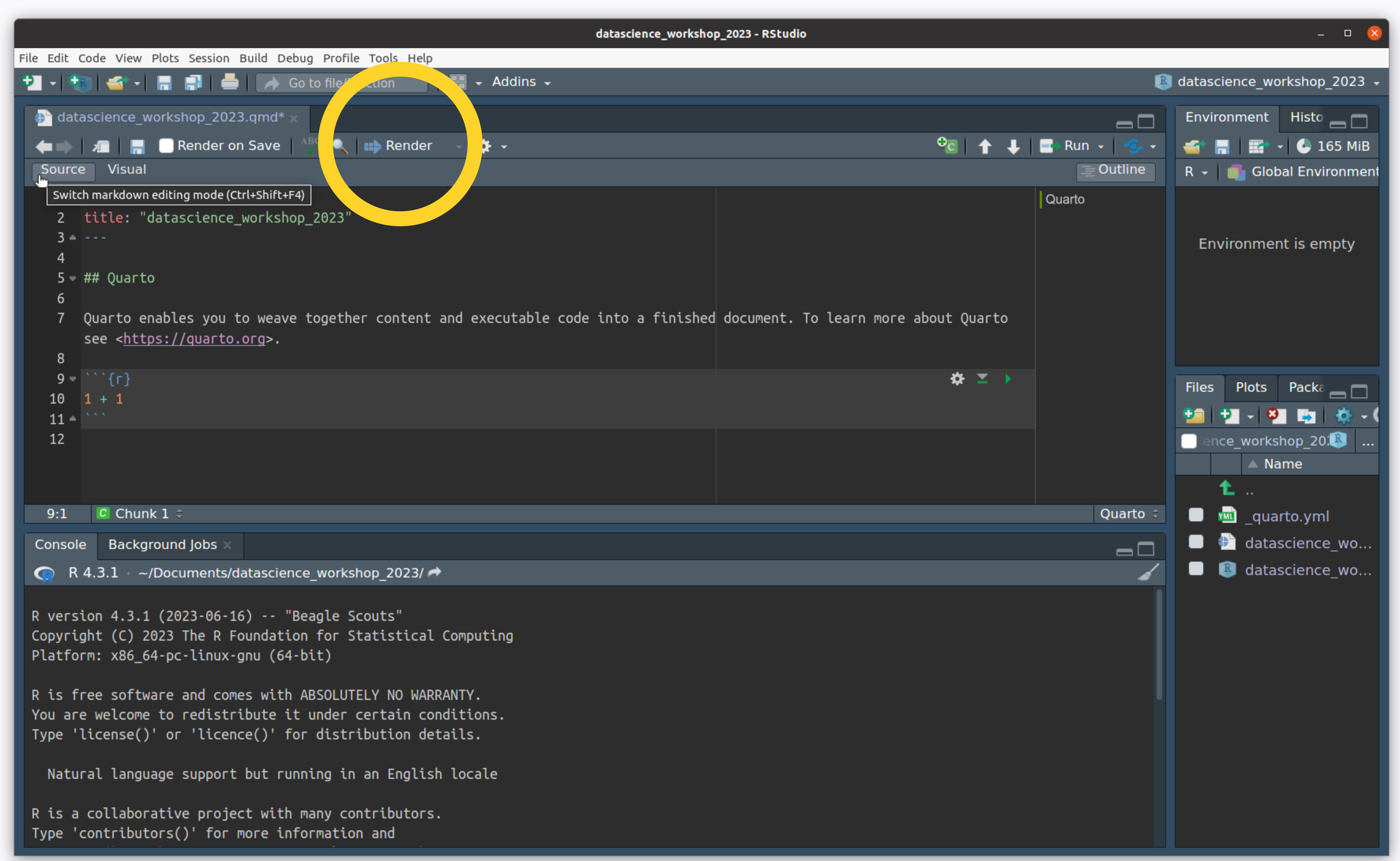
- Switch from “visual” to “source” to see the plain-text version of this document.
Create an R Project
- Click on “Render” to ask Quarto to turn this plain-text document into an HTML page
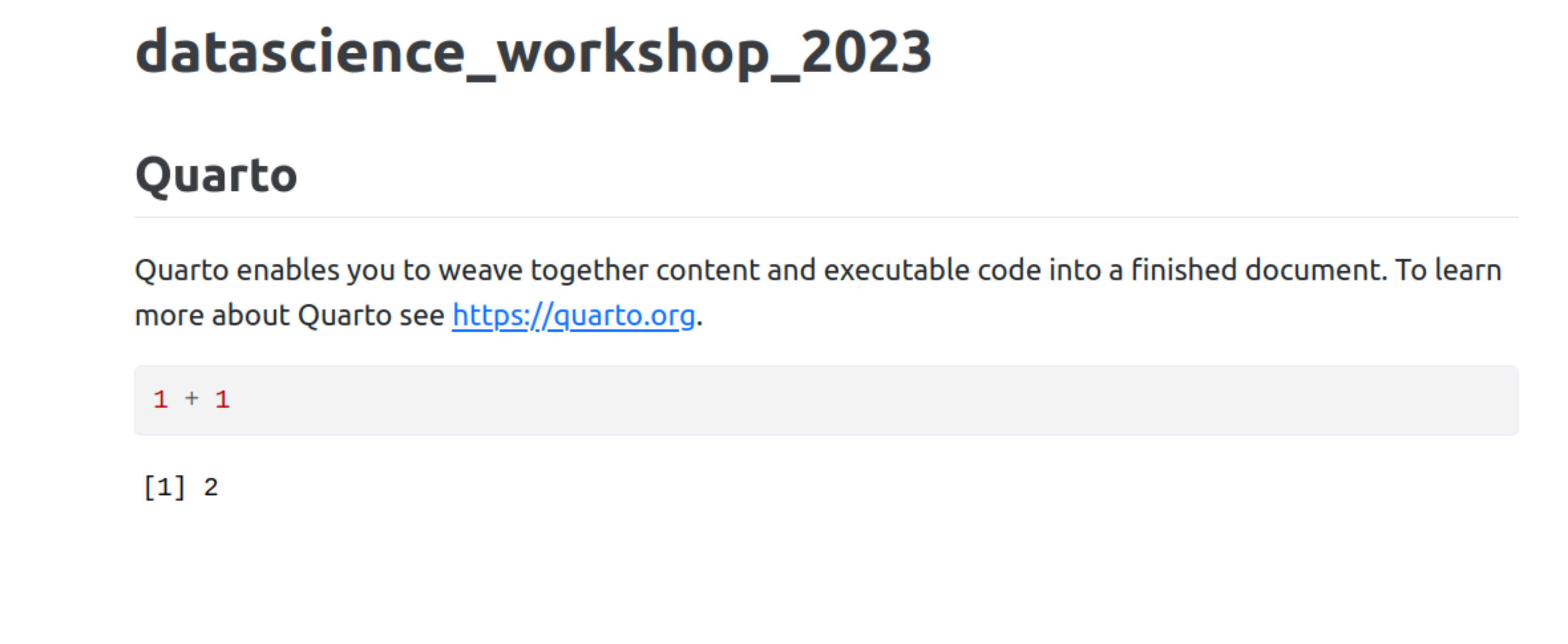
Create an R Project
- Your default web-browser will open and show you the rendered document!
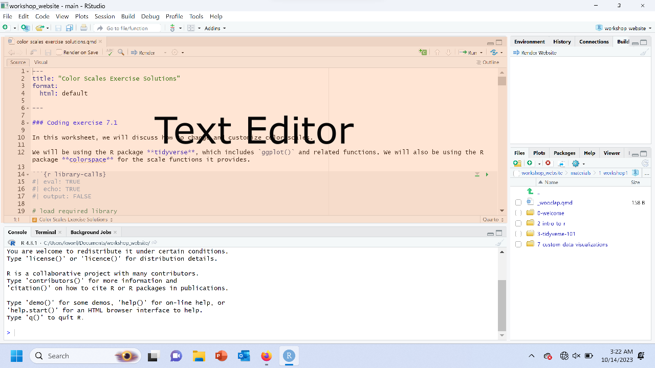
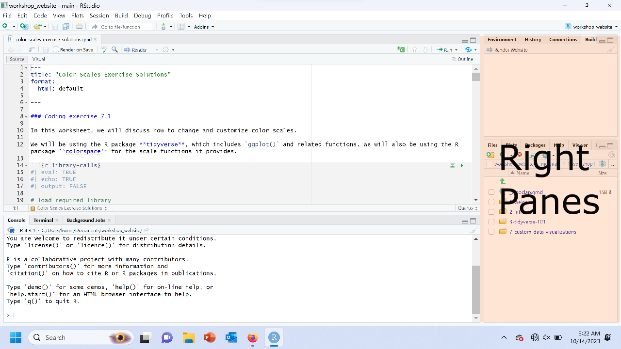
The text editor
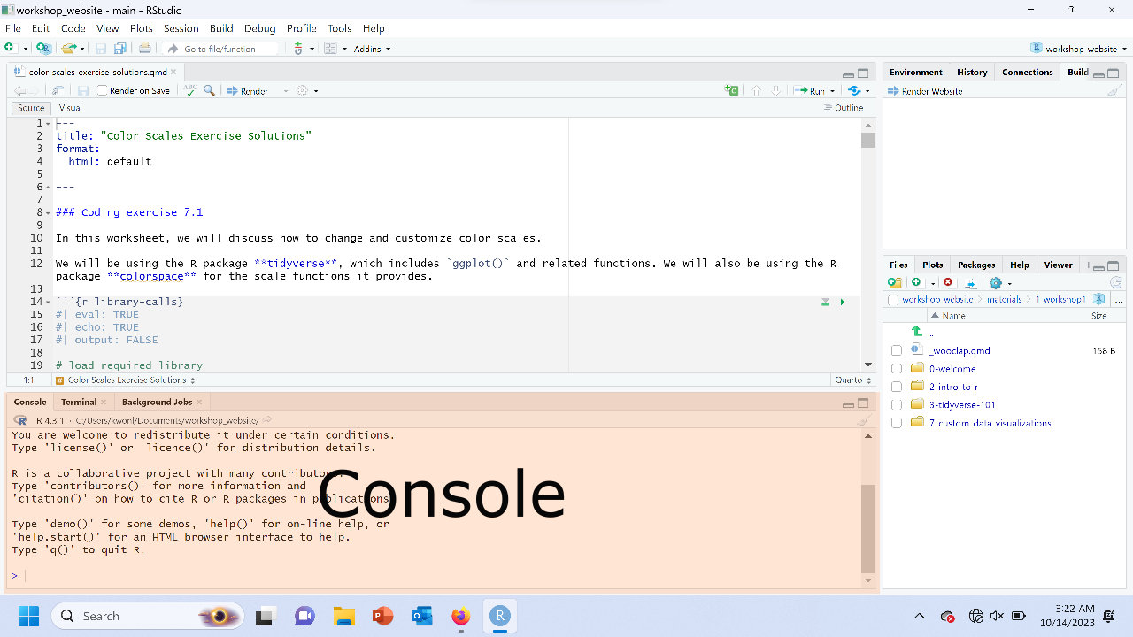
The console
The right panes
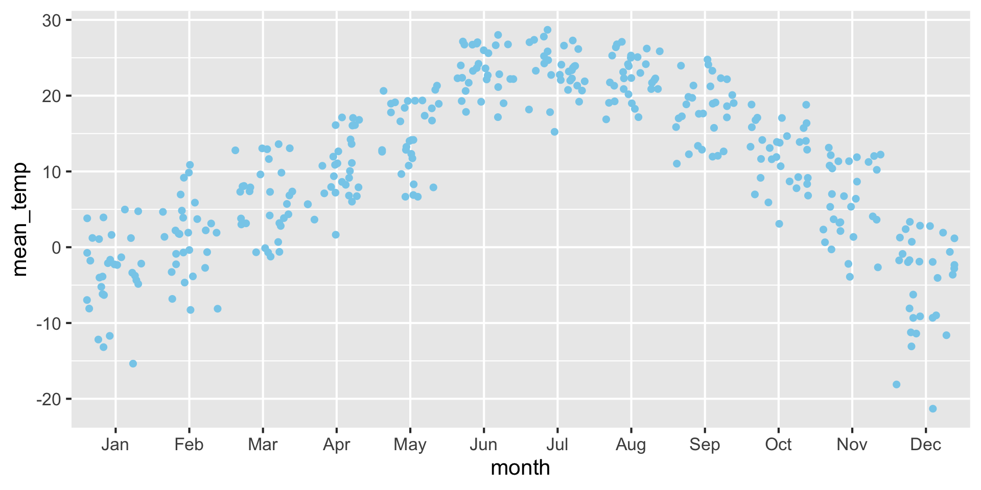
Example: Figures from Code
Inline Elements: Links and Images
Markdown
You can embed [links with names](https://quarto.org/), direct urls
like <https://quarto.org/>, and links to
[other places](#inline-elements-text-formatting) in the document.
The syntax is similar for embedding an inline image:
.
Output
You can embed links with names, direct urls like https://quarto.org/, and links to other places in the document. The syntax is similar for embedding an inline image: ![]() .
.
The pipe %>% feeds data into functions
The pipe %>% feeds data into functions

Pick rows from a table: filter()

Pick columns from a table: select()

Sort the rows in a table: arrange()

Let’s take a poll
Go to the event on wooclap
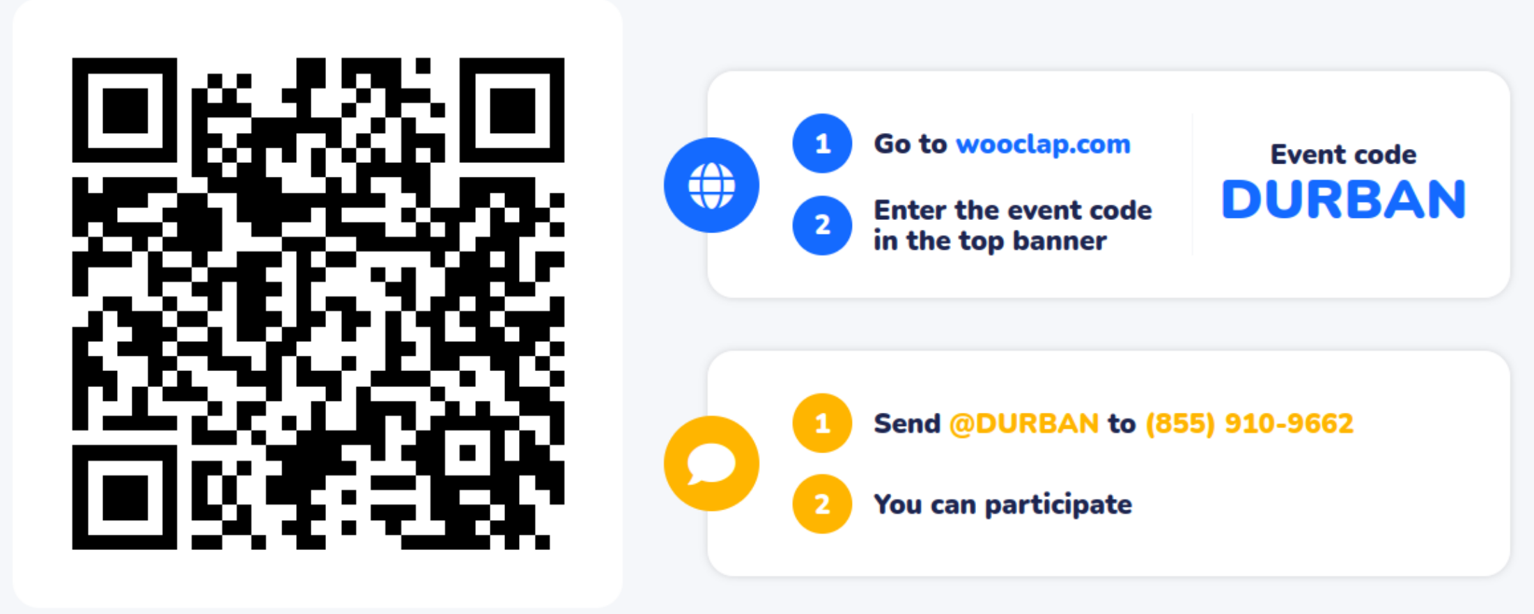
M2. Does filter get rid of rows that match TRUE, or keep rows that match TRUE?
Make a new table column: mutate()

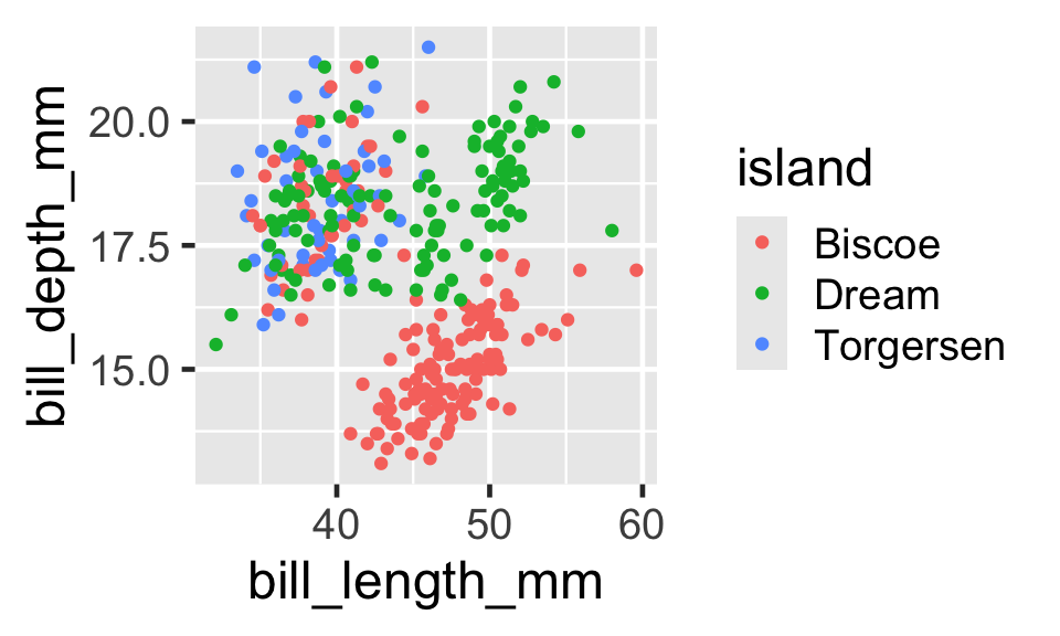
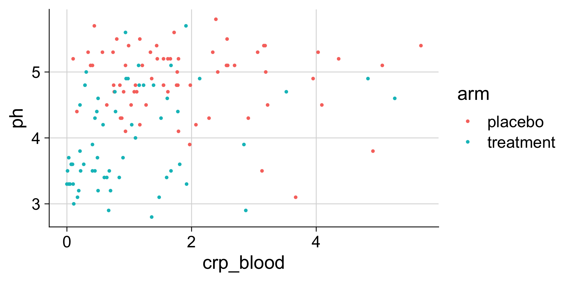
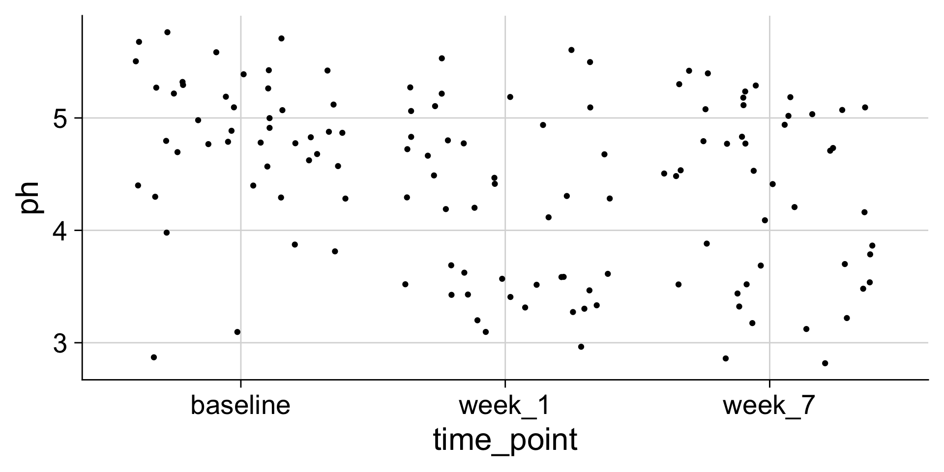
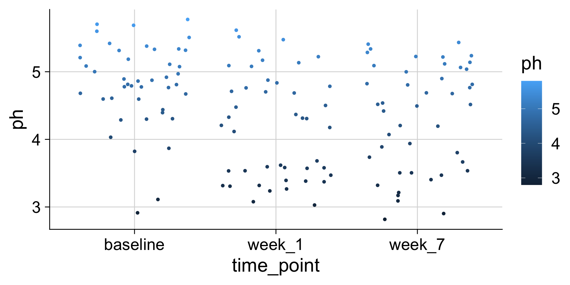
pH mapped to y position
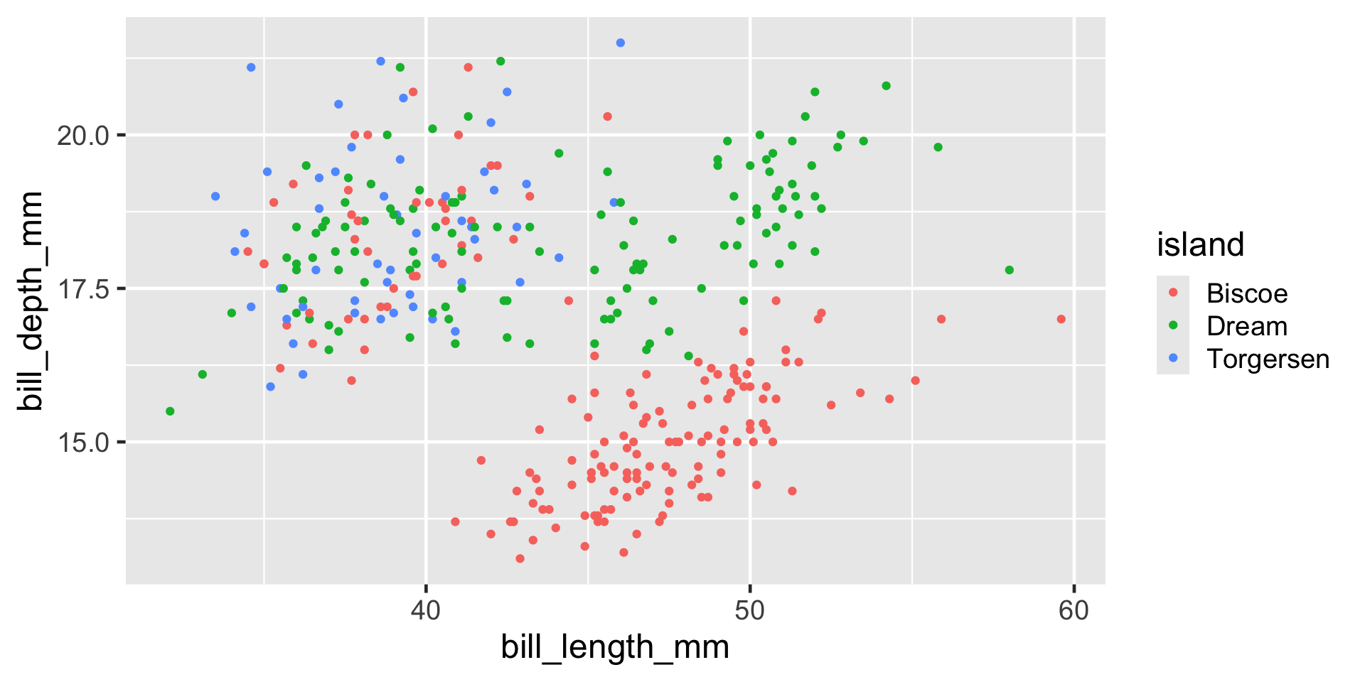
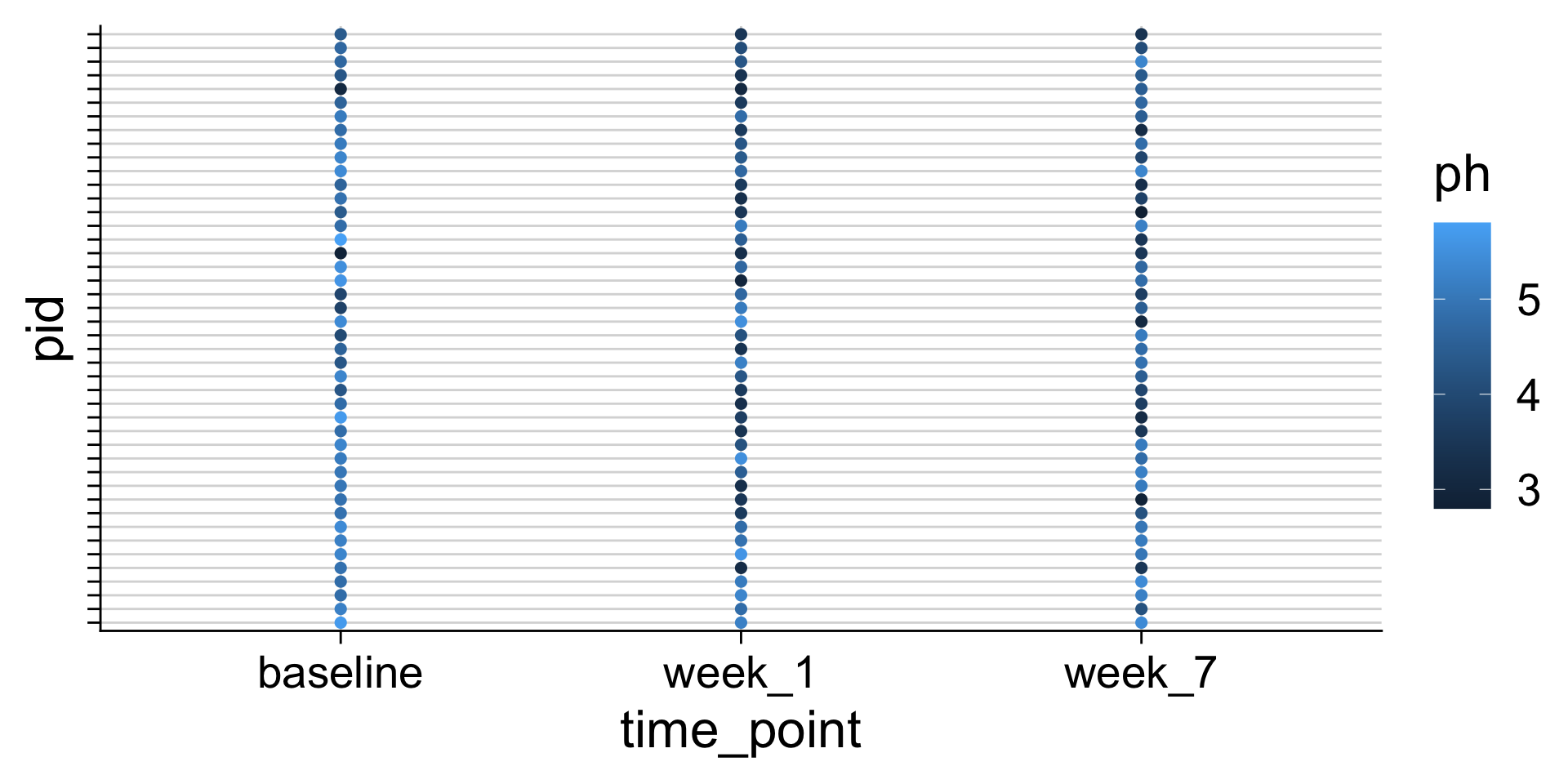
pH mapped to color
Commonly used aesthetics

Figure from Claus O. Wilke. Fundamentals of Data Visualization. O’Reilly, 2019
The same data values can be mapped to different aesthetics

Figure from Claus O. Wilke. Fundamentals of Data Visualization. O’Reilly, 2019
We can use many different aesthetics at once

We define the mapping with aes()
The geom determines how the data is shown
The geom determines how the data is shown
The geom determines how the data is shown
Different geoms have parameters for control
Different geoms have parameters for control
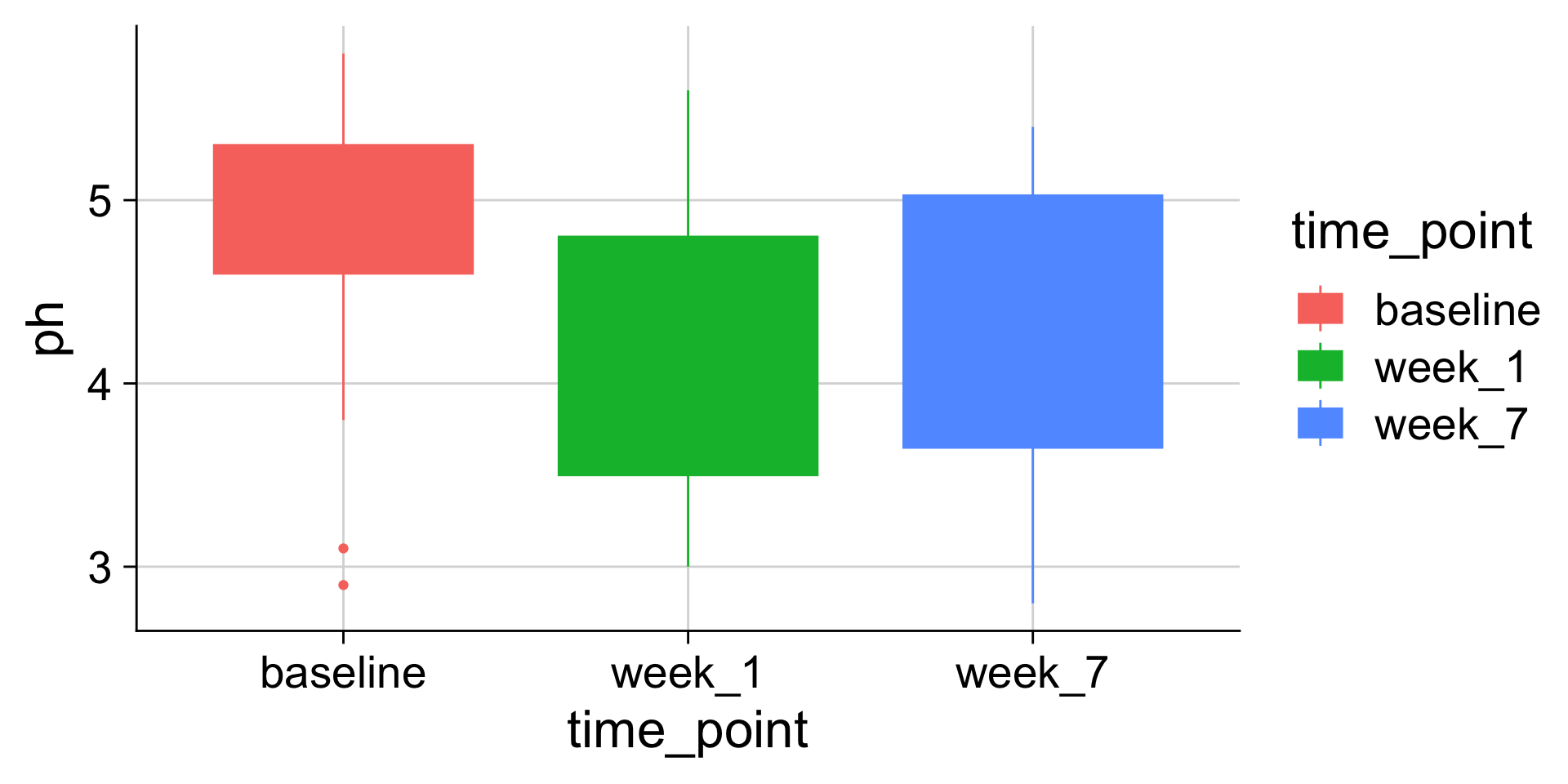
Many geoms have both color and fill aesthetics
Many geoms have both color and fill aesthetics
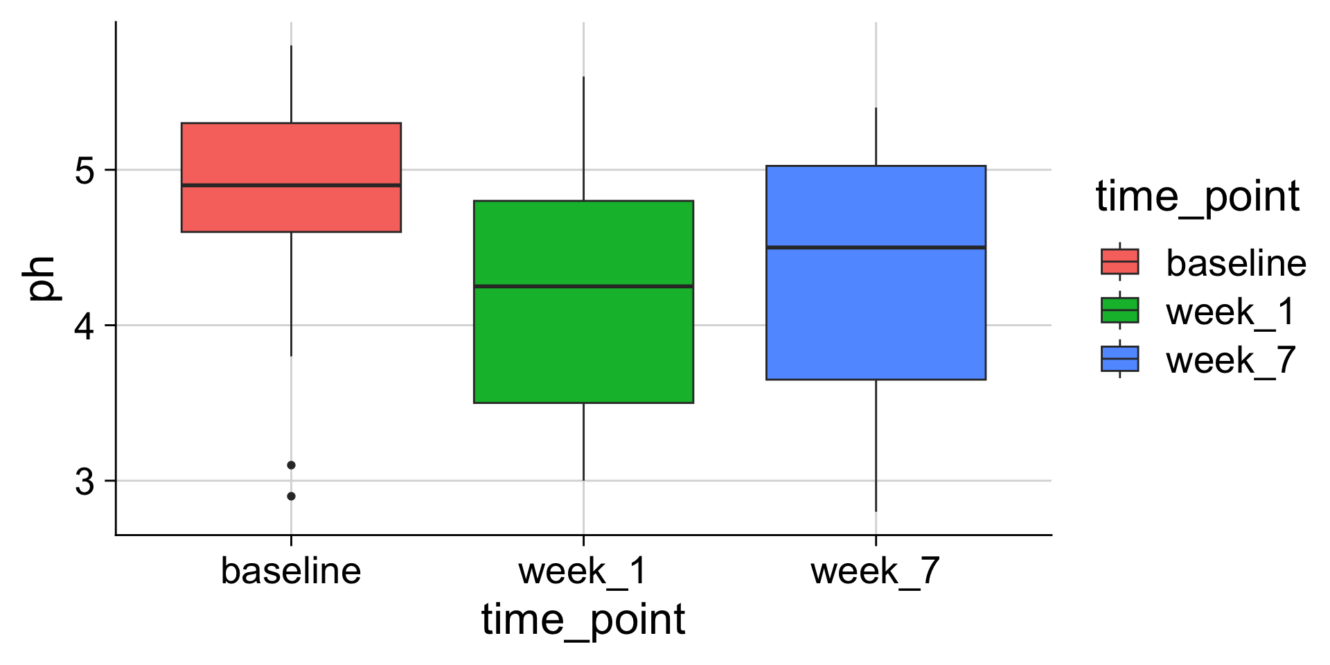
Many geoms have both color and fill aesthetics
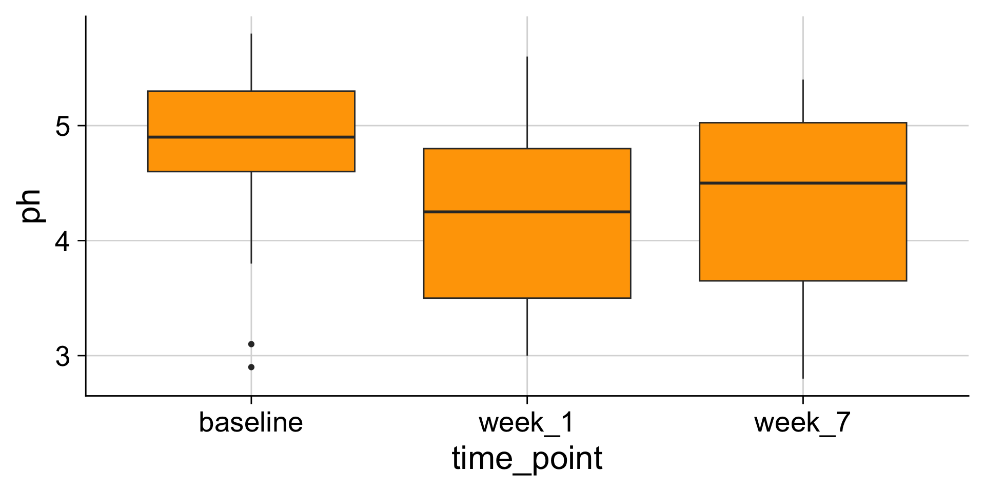
Aesthetics can also be used as parameters in geoms

Aesthetics can also be used as parameters in geoms
Analyze subsets: group_by() and summarize()

Reshape: pivot_wider() and pivot_longer()

We use joins to add columns from one table into another

There are different types of joins
The differences are all about how to handle when the two tables have different key values

left_join() - the resulting table always has the same key_values as the “left” table
right_join() - the resulting table always has the same key_values as the “right” table
inner_join() - the resulting table always only keeps the key_values that are in both tables
full_join() - the resulting table always has all key_values found in both tables
Left Join
left_join() - the resulting table always has the same key_values as the “left” table

inner_join
inner_join() - the resulting table always only keeps the key_values that are in both tables

Note, merging tables vertically is bind_rows(), not a join

Histograms depend on the chosen bin width

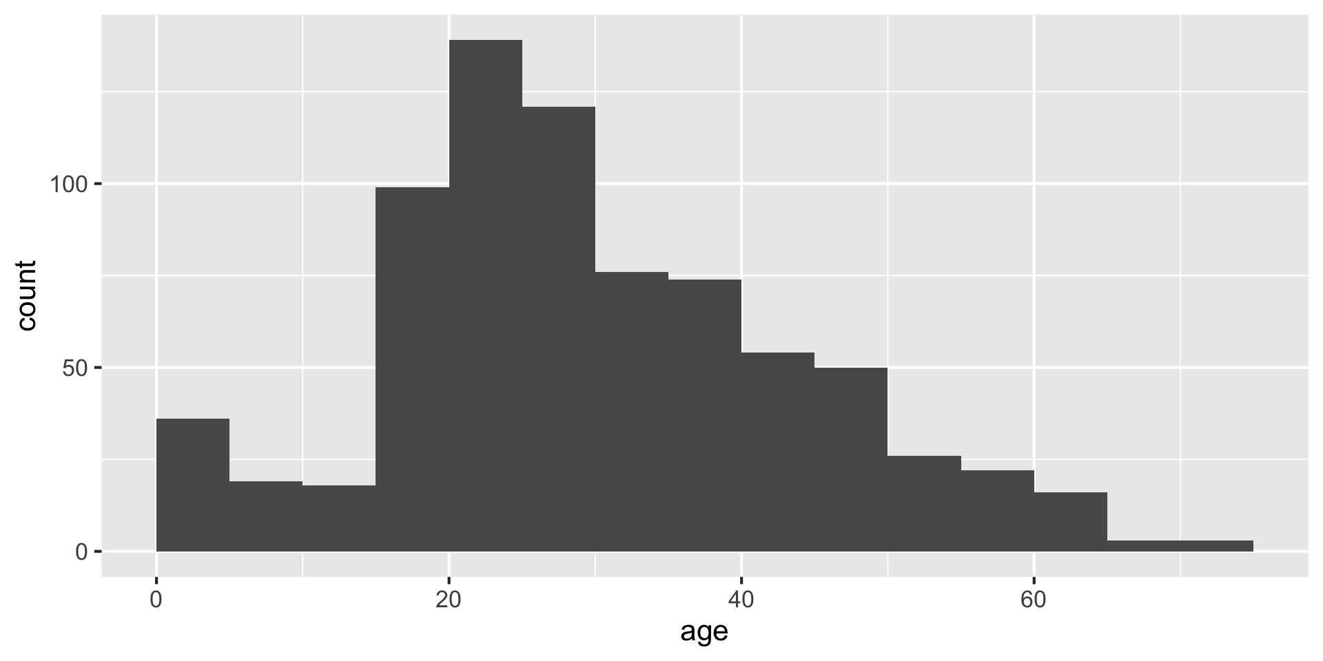
Making histograms with ggplot: geom_histogram()
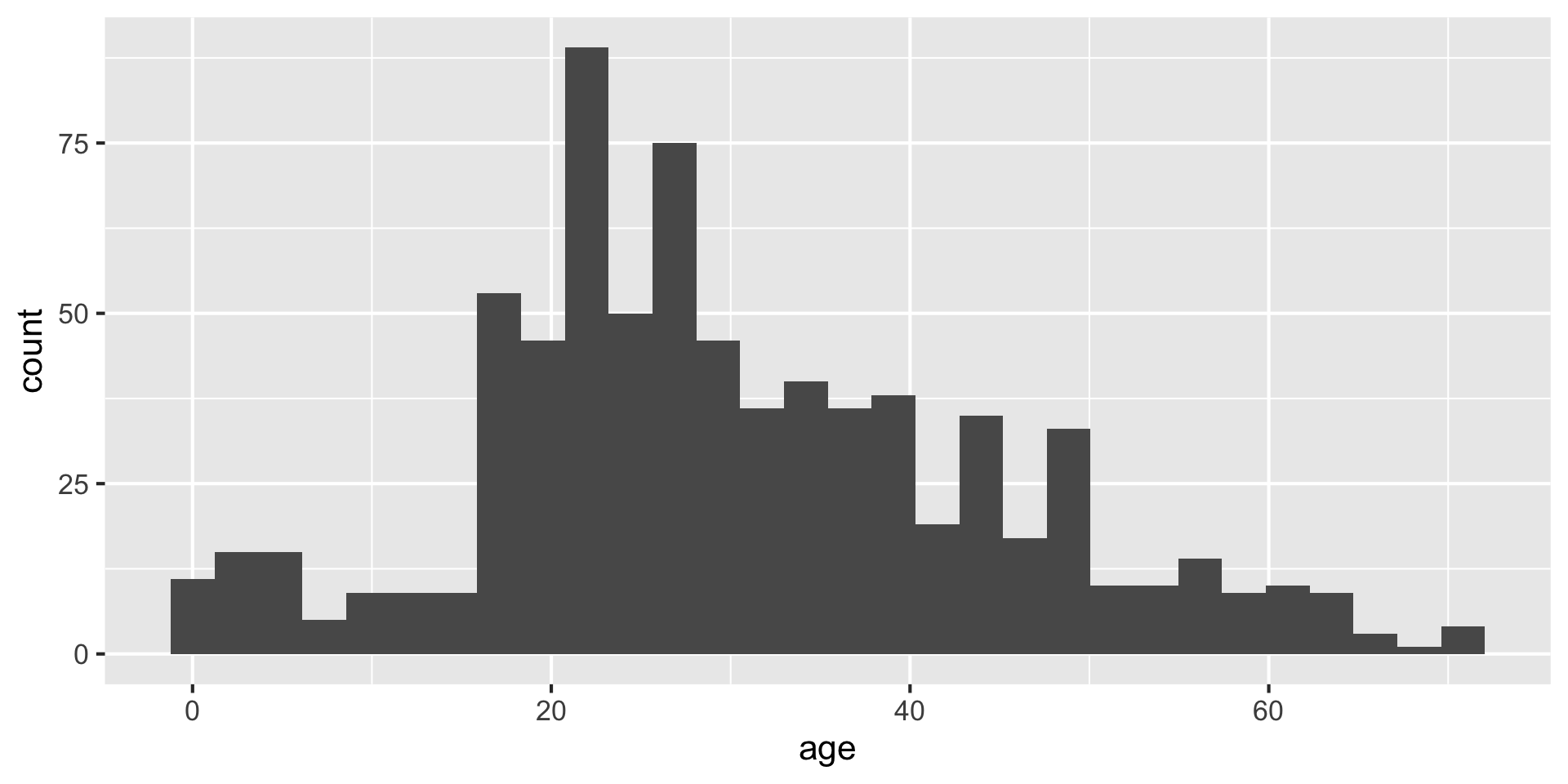
Setting the bin width
Do you like where there bins are? What does the first bin say?
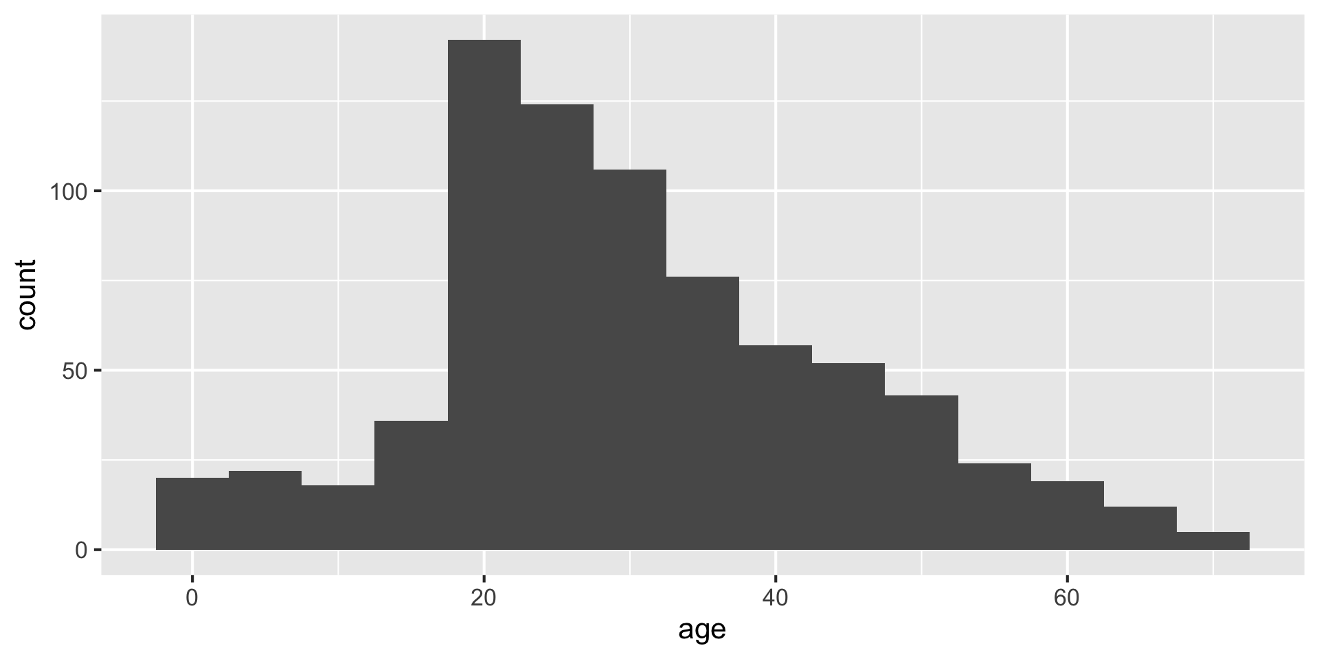
Always set the center as well, to half the bin_width
Setting center 2.5 makes the bars start 0-5, 5-10, etc. instead of 2.5-7.5, etc. You could instead use the argument boundary=5 to accomplish the same behavior.
Making density plots with ggplot: geom_density()
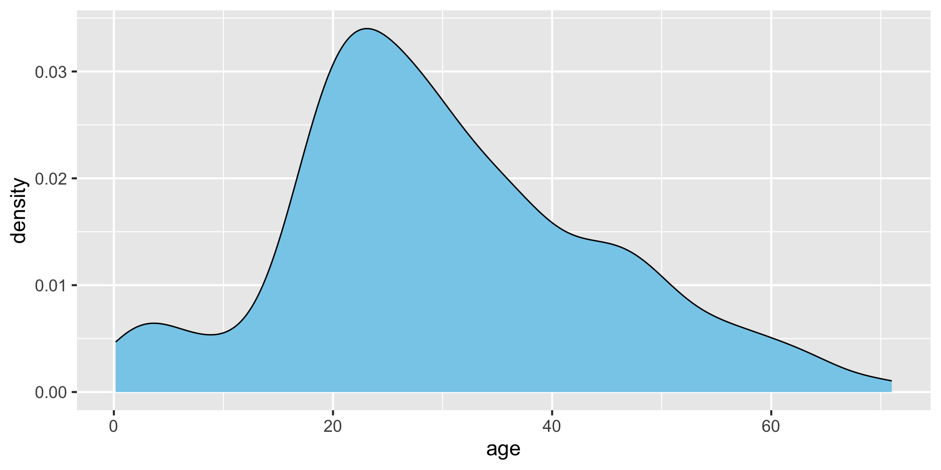
Making density plots with ggplot: geom_density()
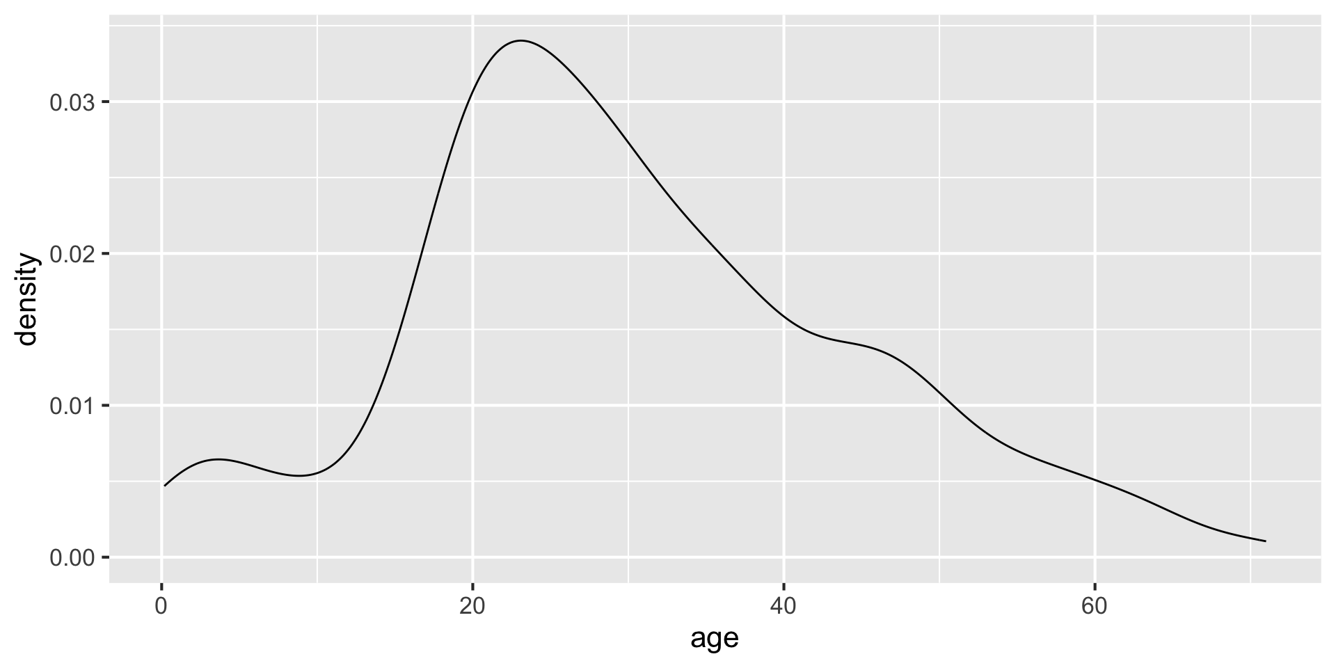
without fill
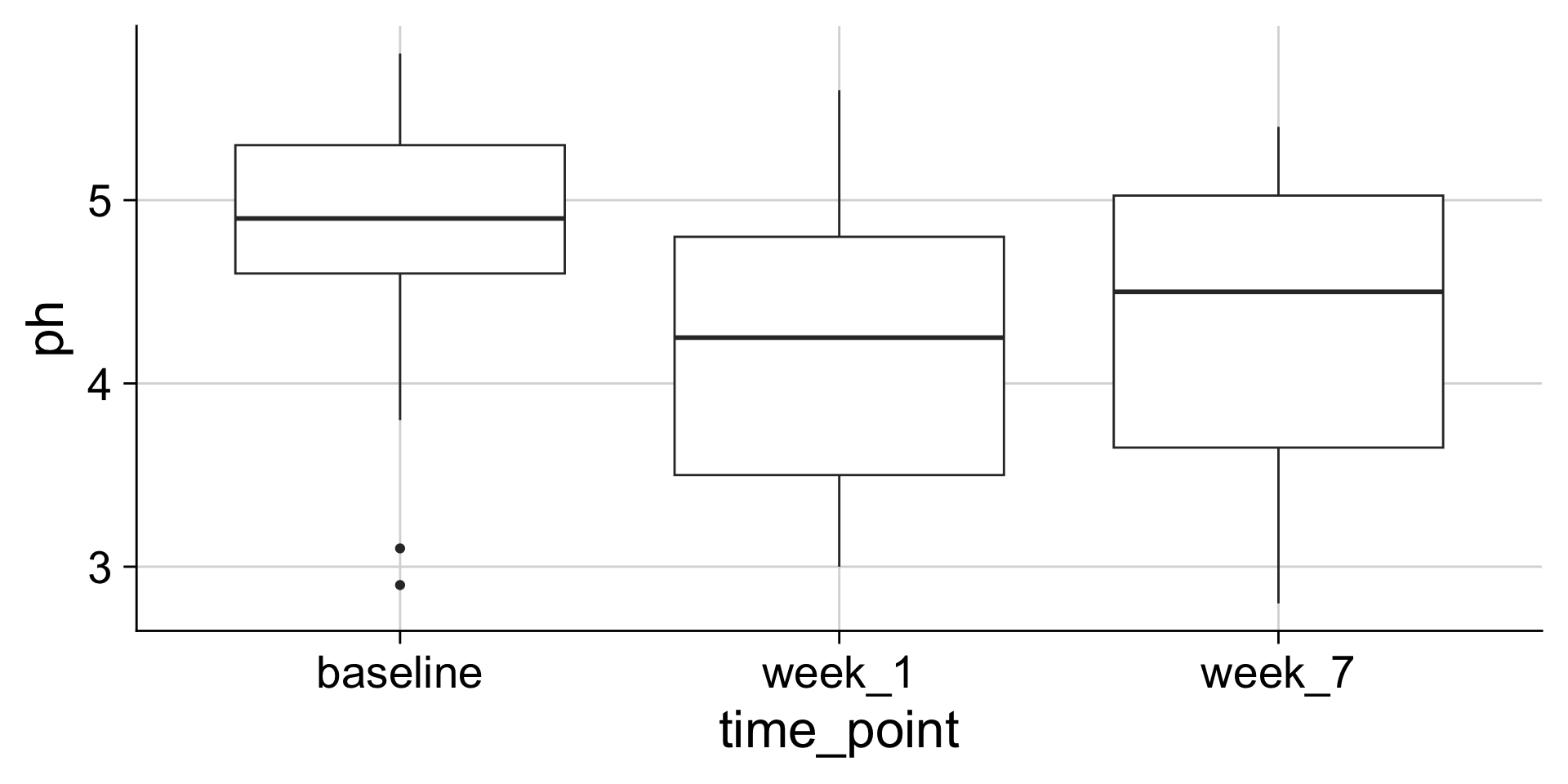
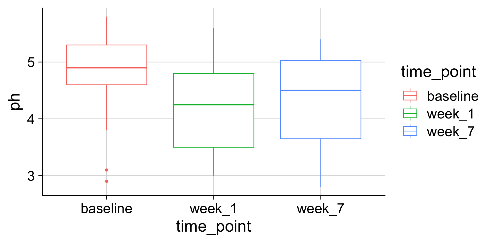
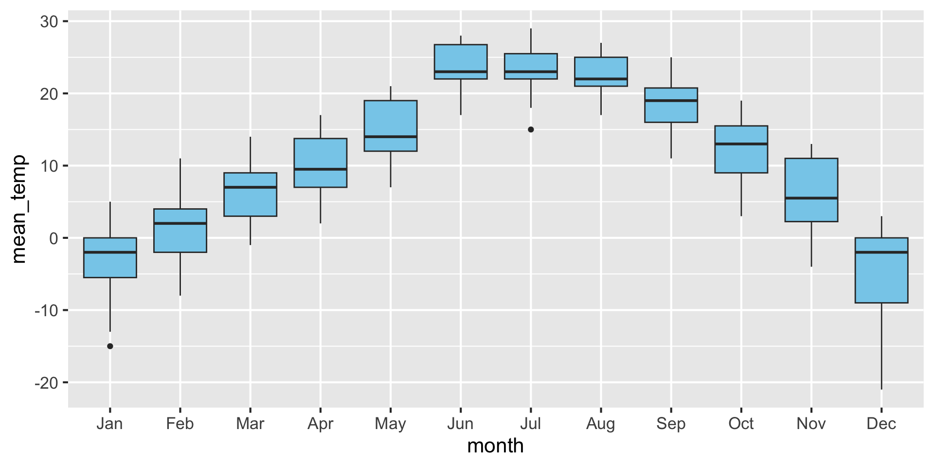
Boxplots: Showing values along y, conditions along x
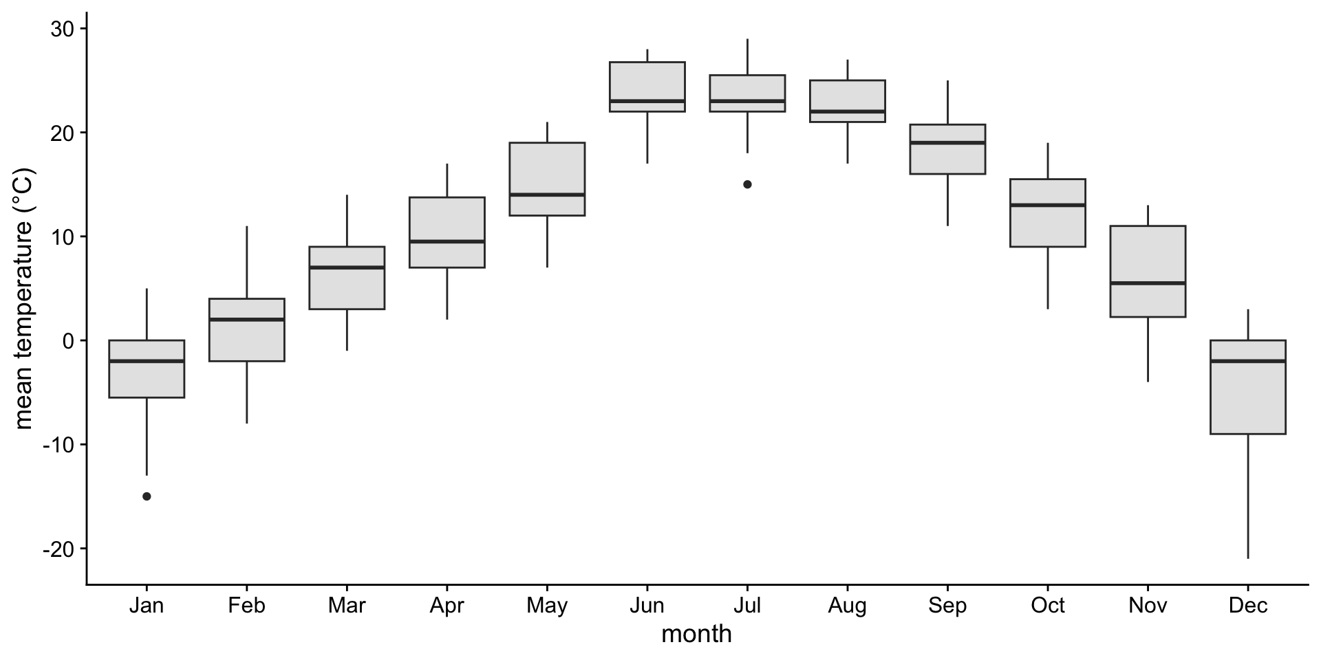
A boxplot is a crude way of visualizing a distribution.
How to read a boxplot

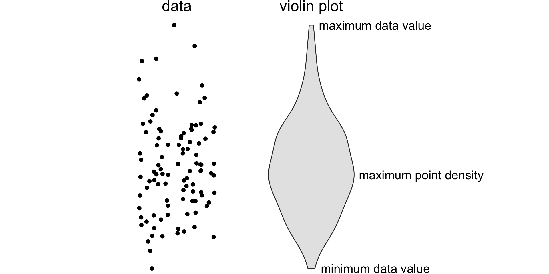
If you like density plots, consider violins
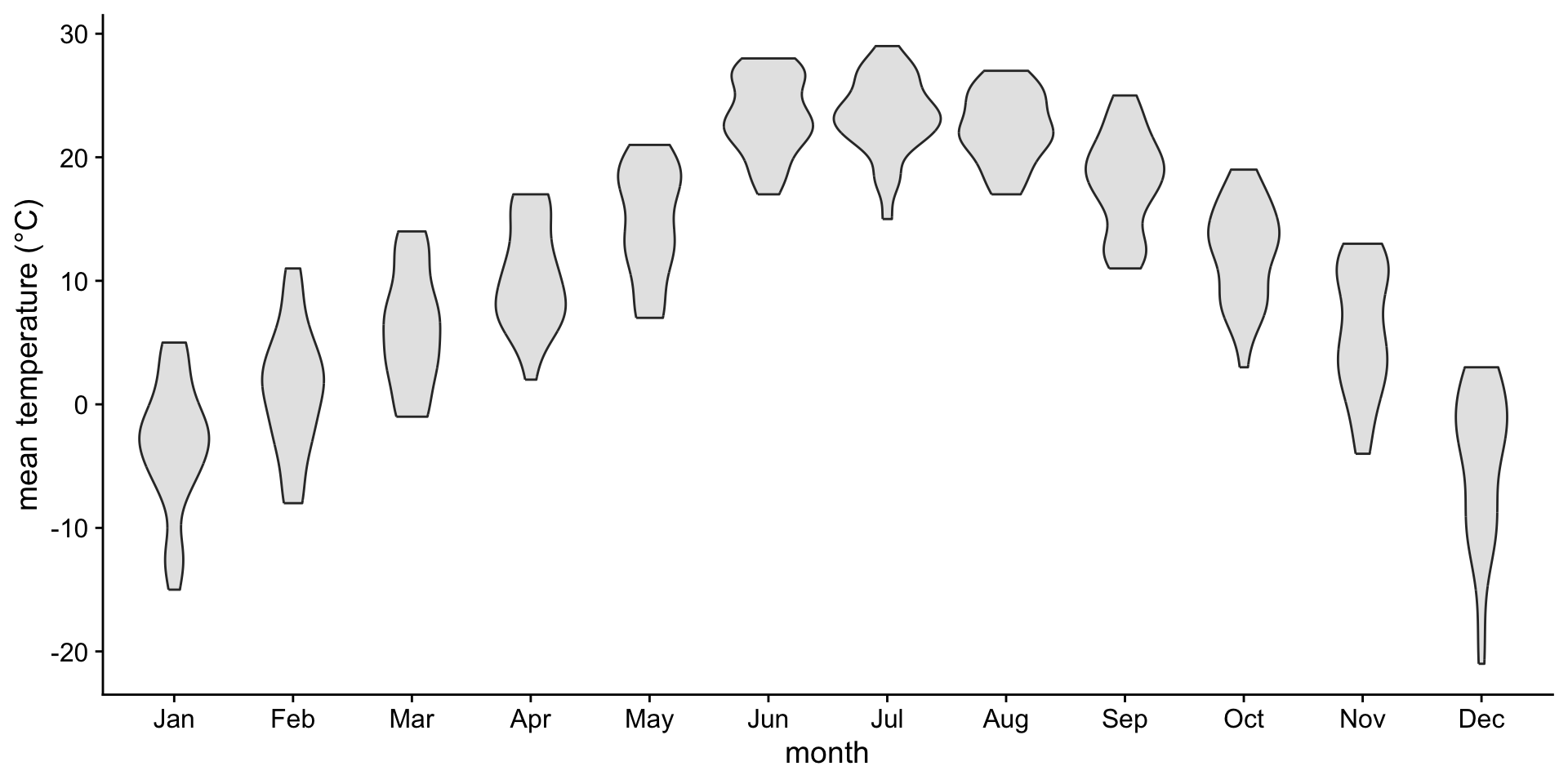
A violin plot is a density plot rotated 90 degrees and then mirrored.
How to read a violin plot
Examples: Boxplot
Examples: Violins

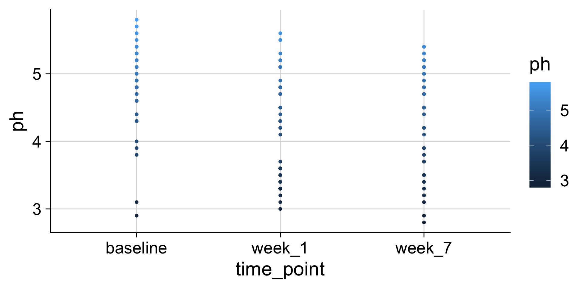
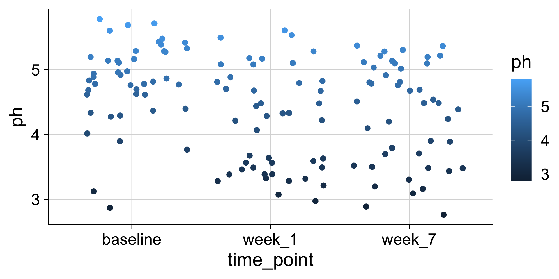
Examples: Strip chart (no jitter)
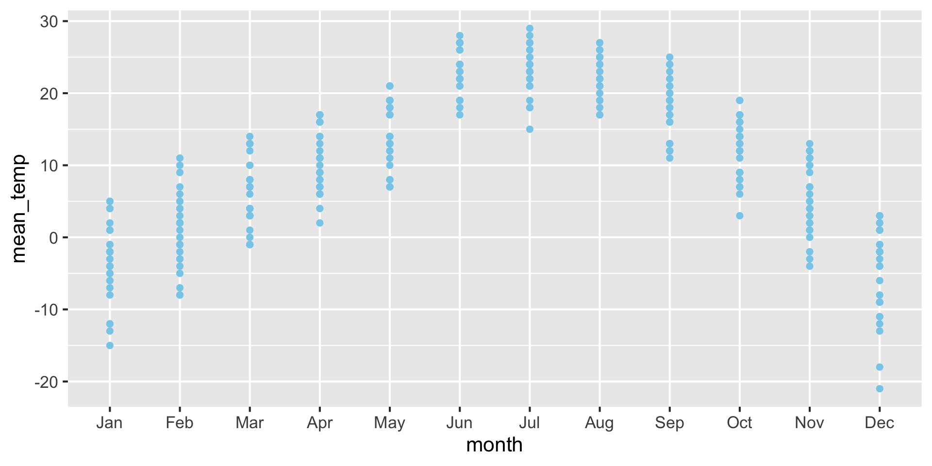
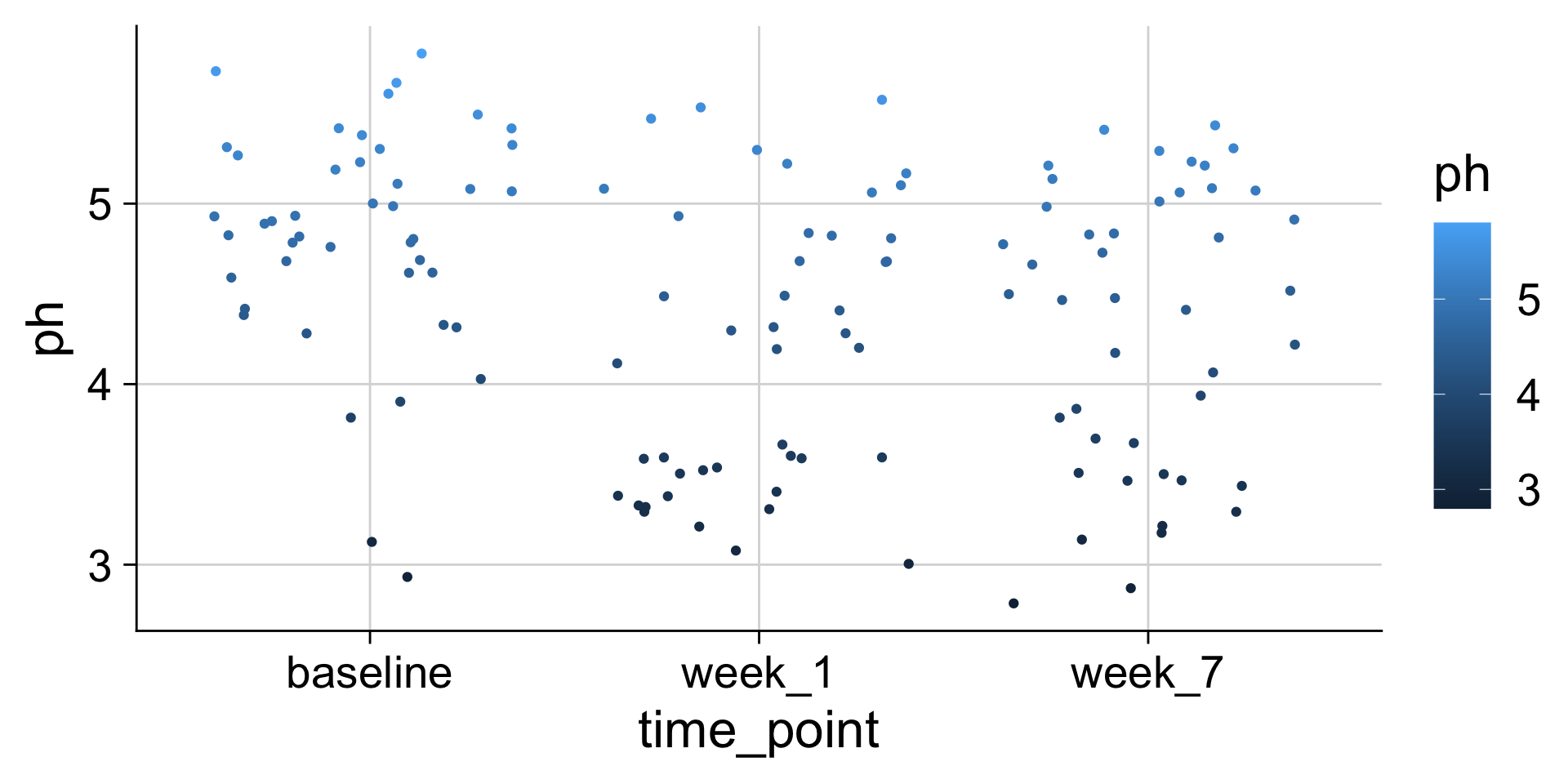
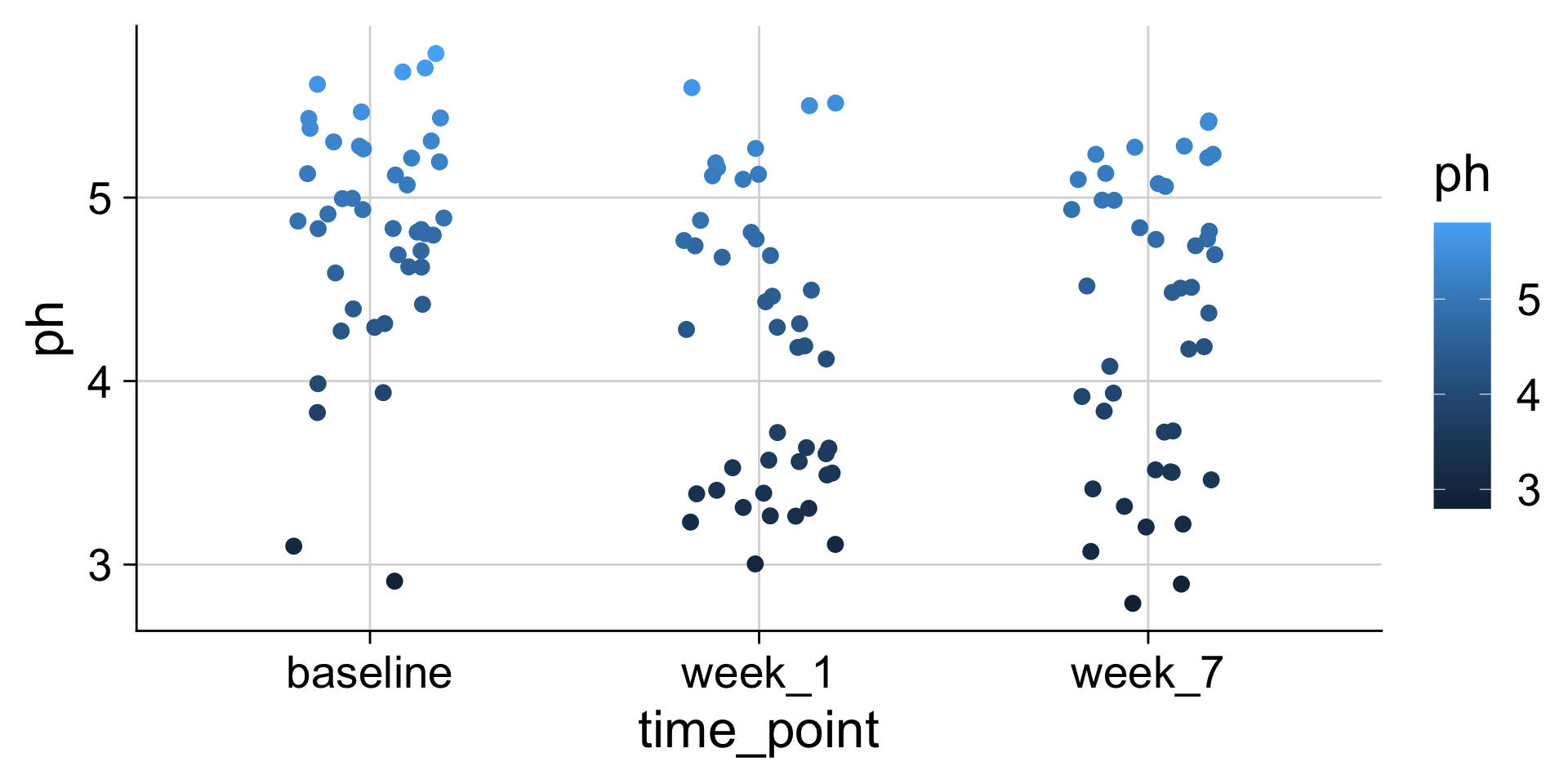
Examples: Strip chart (w/ jitter)