Figure Design
remixed from Claus O. Wilke’s SDS375 course
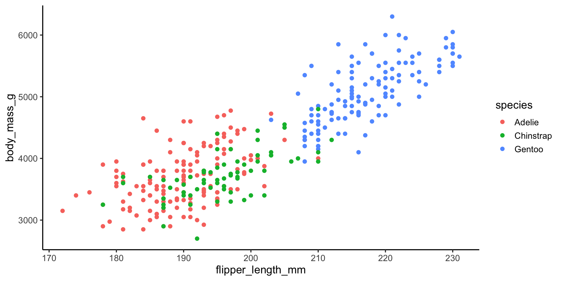
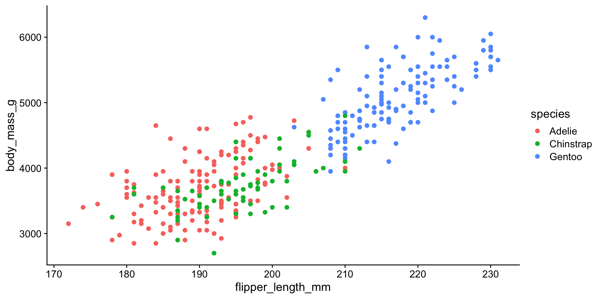
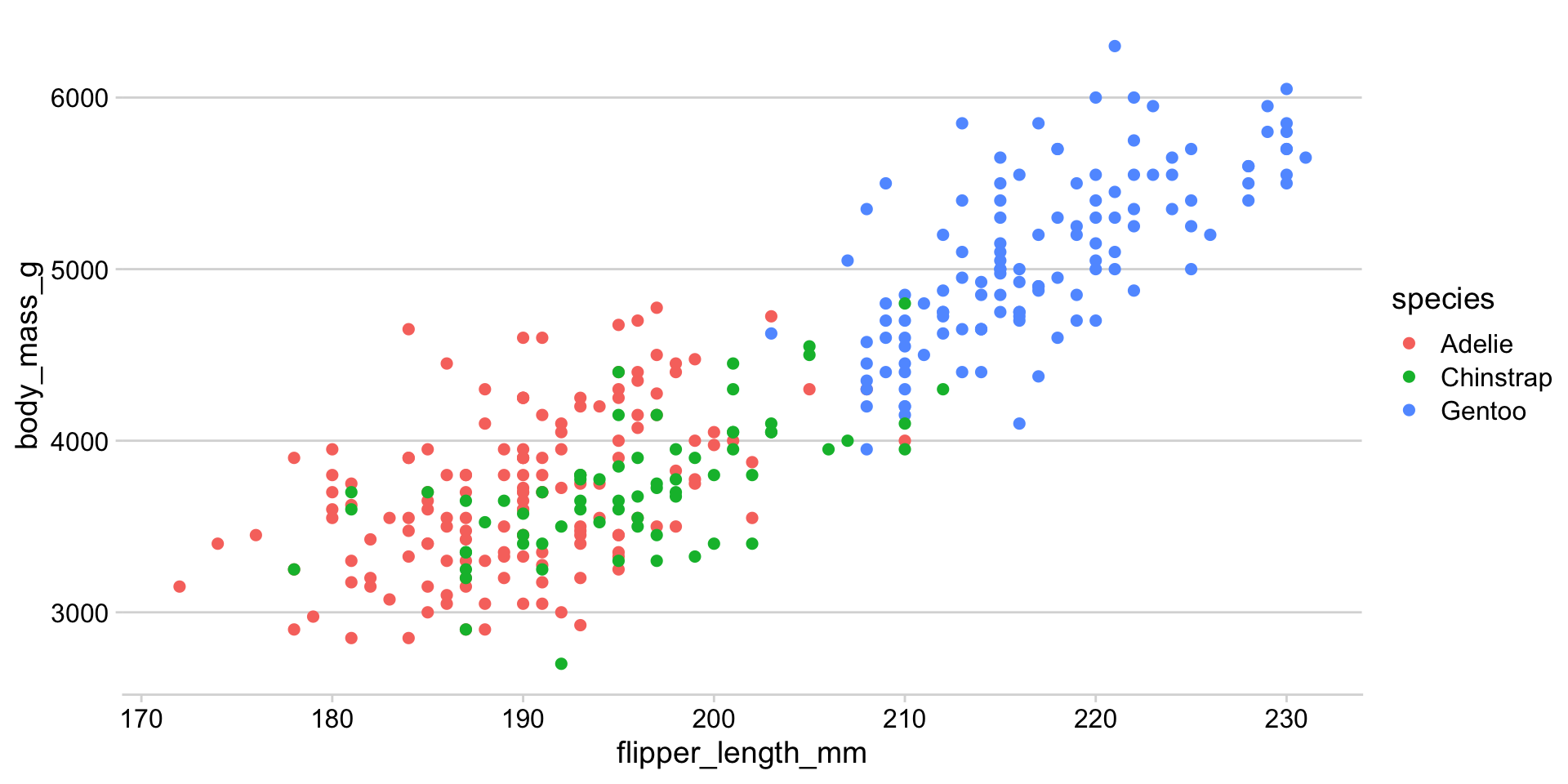
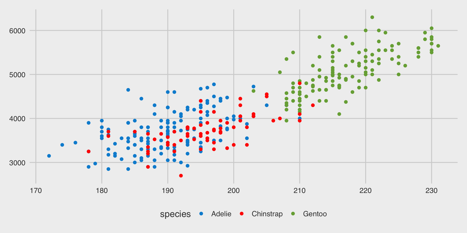
How to go from this …
… to this?

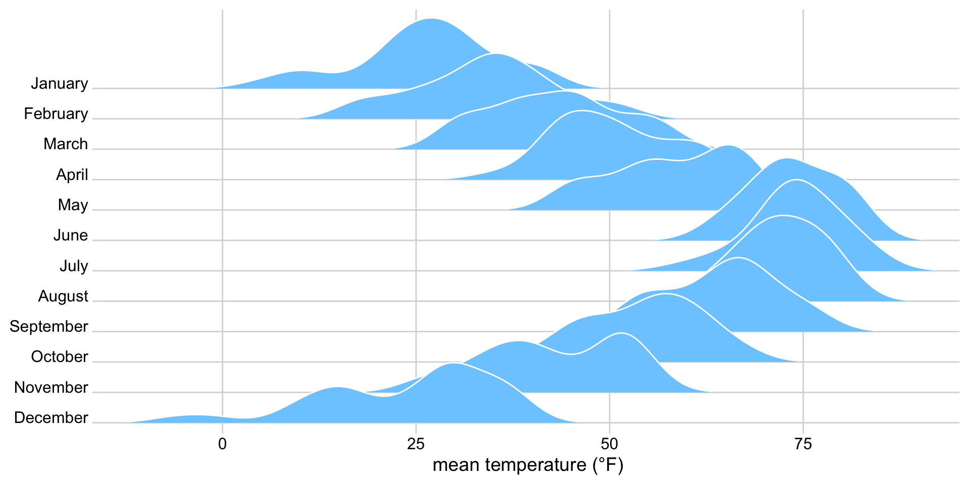
Requires coordinated modification of multiple elements:
- geoms (via arguments to geoms)
- scales (via scale_*() functions)
- plot appearance (via themes)
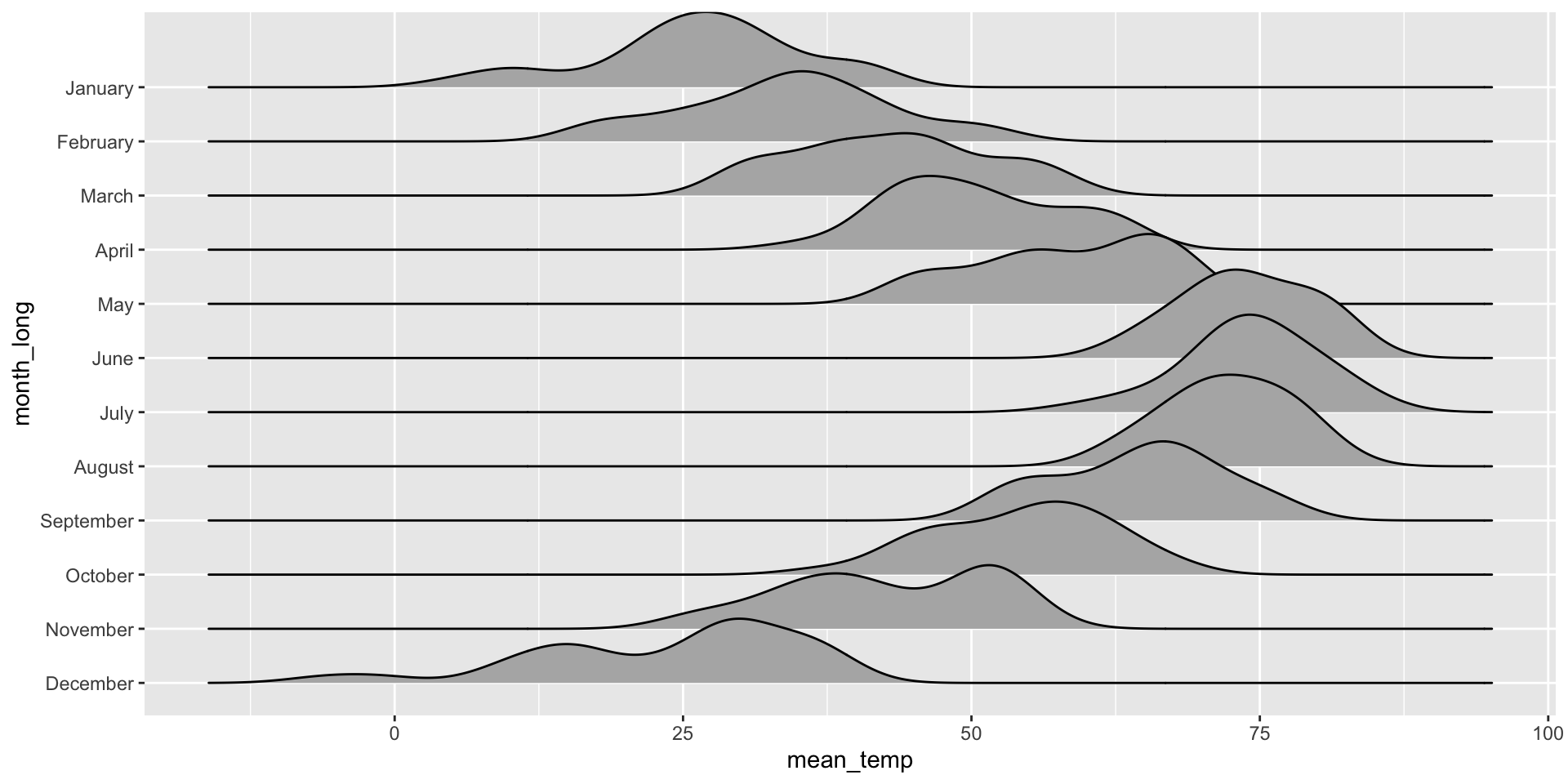
The starting point, a rough draft
ggplot(lincoln_temps) +
  aes(x = mean_temp, y = month_long) +
  geom_density_ridges()
lincoln_temps <- readRDS(
  url("https://wilkelab.org/DSC385/datasets/lincoln_temps.rds")
)
You can download the dataset using this code:
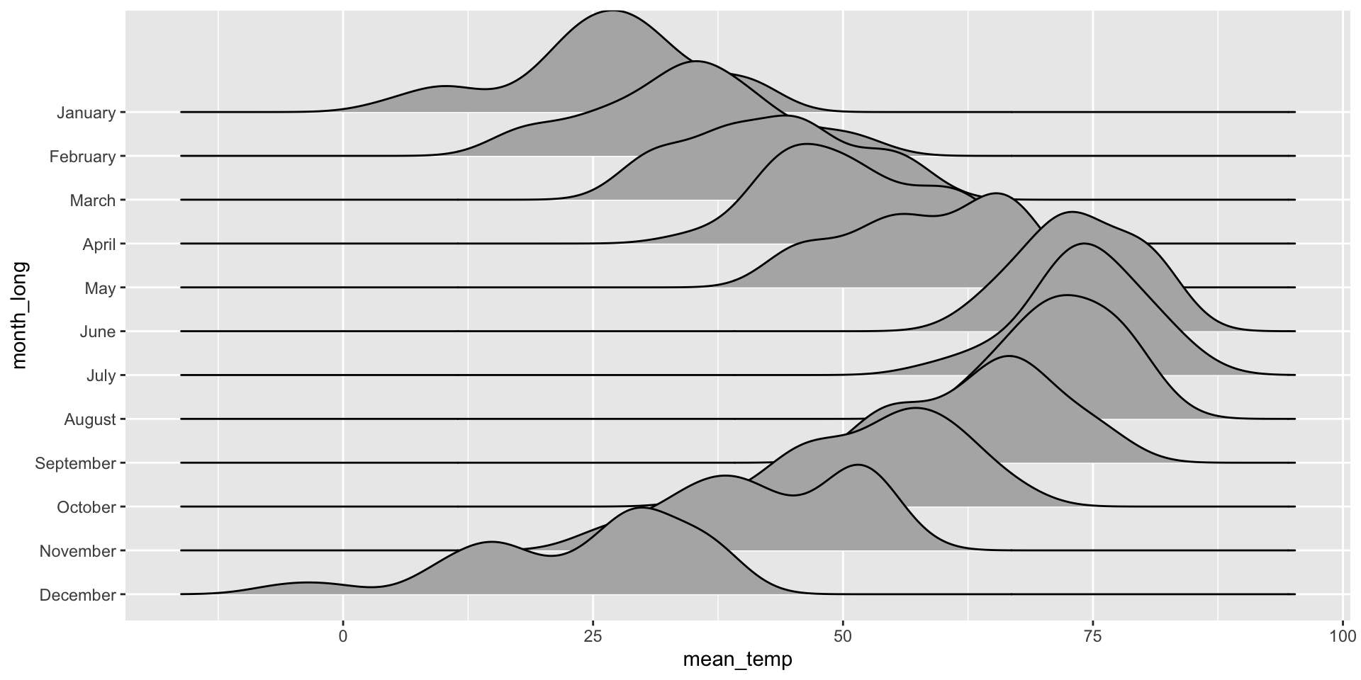
Set scale and bandwidth to shape ridgelines
ggplot(lincoln_temps) +
  aes(x = mean_temp, y = month_long) +
  geom_density_ridges(
    scale = 3, bandwidth = 3.4
  )
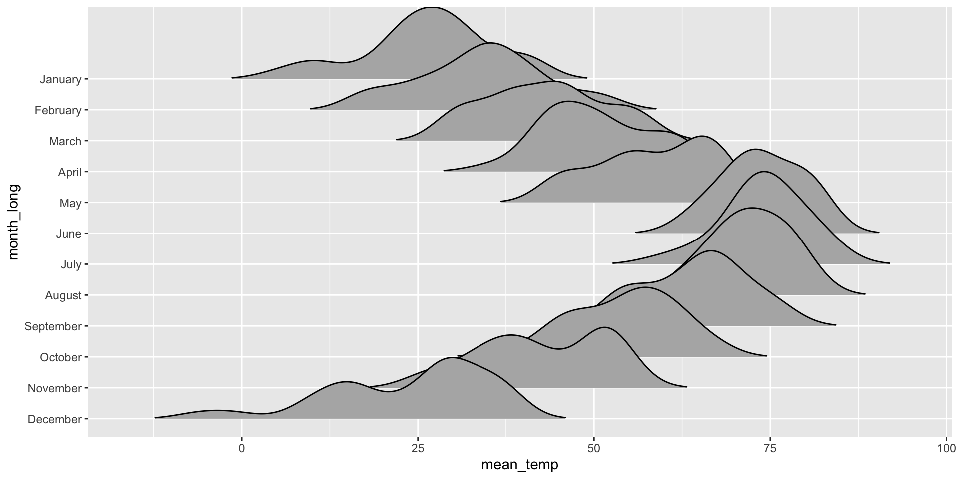
Set rel_min_height to cut ridgelines near zero
ggplot(lincoln_temps) +
  aes(x = mean_temp, y = month_long) +
  geom_density_ridges(
    scale = 3, bandwidth = 3.4,
    rel_min_height = 0.01
  )
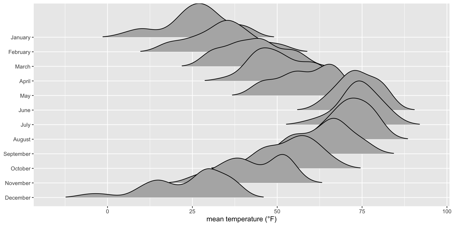
Use scale_*() functions to specify axis labels
ggplot(lincoln_temps) +
  aes(x = mean_temp, y = month_long) +
  geom_density_ridges(
    scale = 3, bandwidth = 3.4,
    rel_min_height = 0.01,
  ) +
  scale_x_continuous(
    name = "mean temperature (°F)"
  ) +
  scale_y_discrete(
    name = NULL  # NULL means no label
  )
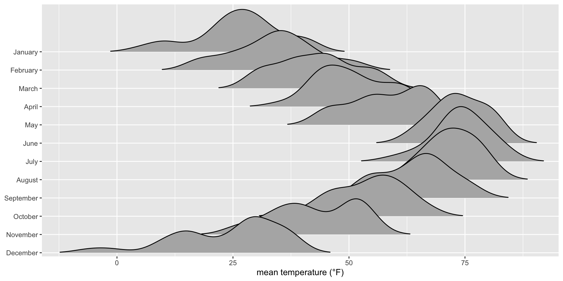
Specify scale expansion
ggplot(lincoln_temps) +
  aes(x = mean_temp, y = month_long) +
  geom_density_ridges(
    scale = 3, bandwidth = 3.4,
    rel_min_height = 0.01
  ) +
  scale_x_continuous(
    name = "mean temperature (°F)",
    expand = c(0, 0)
  ) +
  scale_y_discrete(
    name = NULL,
    expand = expansion(add = c(0.2, 2.6))
  )
Set overall plot theme
ggplot(lincoln_temps) +
  aes(x = mean_temp, y = month_long) +
  geom_density_ridges(
    scale = 3, bandwidth = 3.4,
    rel_min_height = 0.01
  ) +
  scale_x_continuous(
    name = "mean temperature (°F)",
    expand = c(0, 0)
  ) +
  scale_y_discrete(
    name = NULL,
    expand = expansion(add = c(0.2, 2.6))
  ) +
  theme_minimal_grid()  # from cowplot
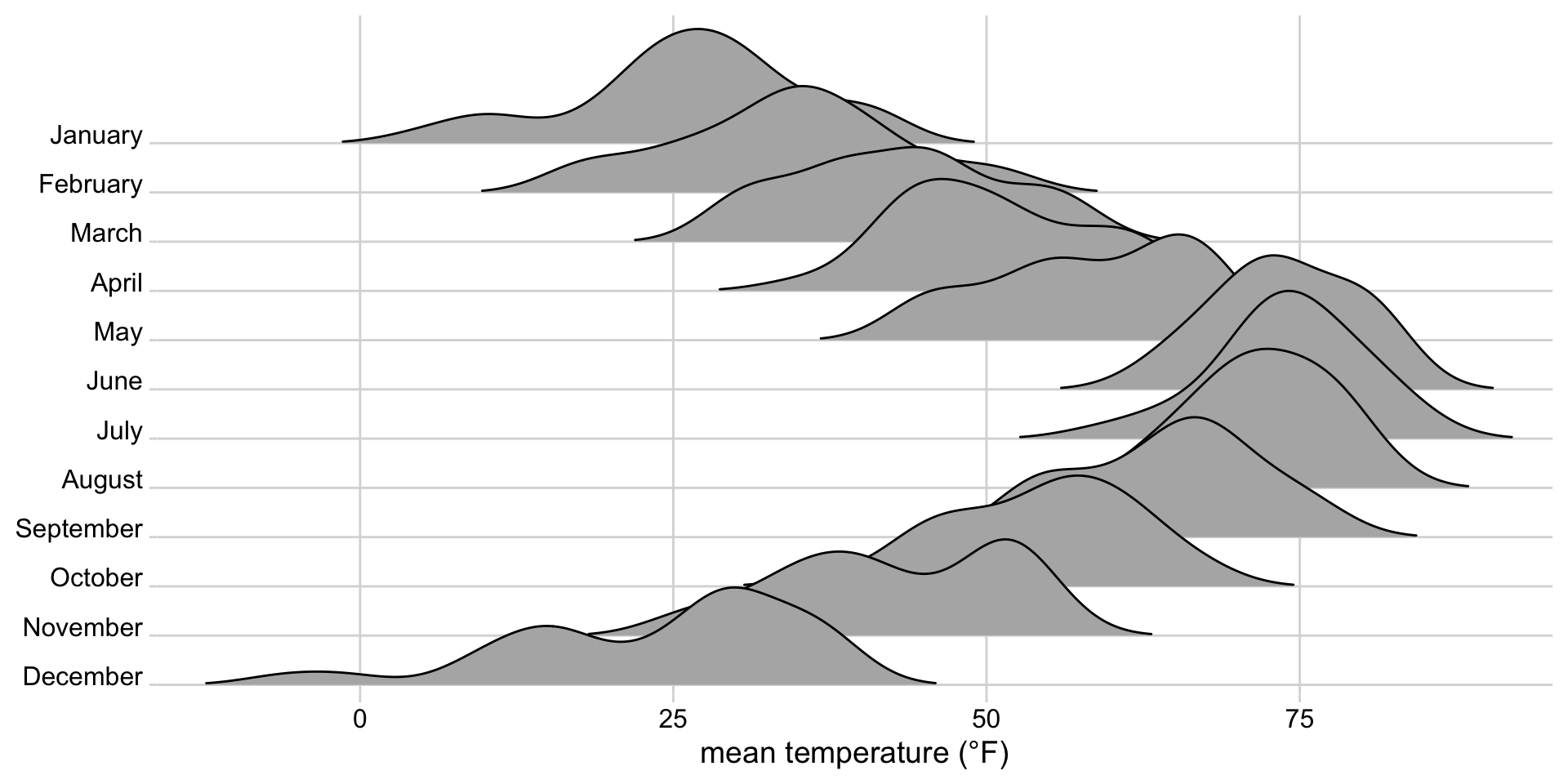
Align y axis labels to grid lines
ggplot(lincoln_temps) +
  aes(x = mean_temp, y = month_long) +
  geom_density_ridges(
    scale = 3, bandwidth = 3.4,
    rel_min_height = 0.01
  ) +
  scale_x_continuous(
    name = "mean temperature (°F)",
    expand = c(0, 0)
  ) +
  scale_y_discrete(
    name = NULL,
    expand = expansion(add = c(0.2, 2.6))
  ) +
  theme_minimal_grid() +
  theme(
    axis.text.y = element_text(vjust = 0)
  )
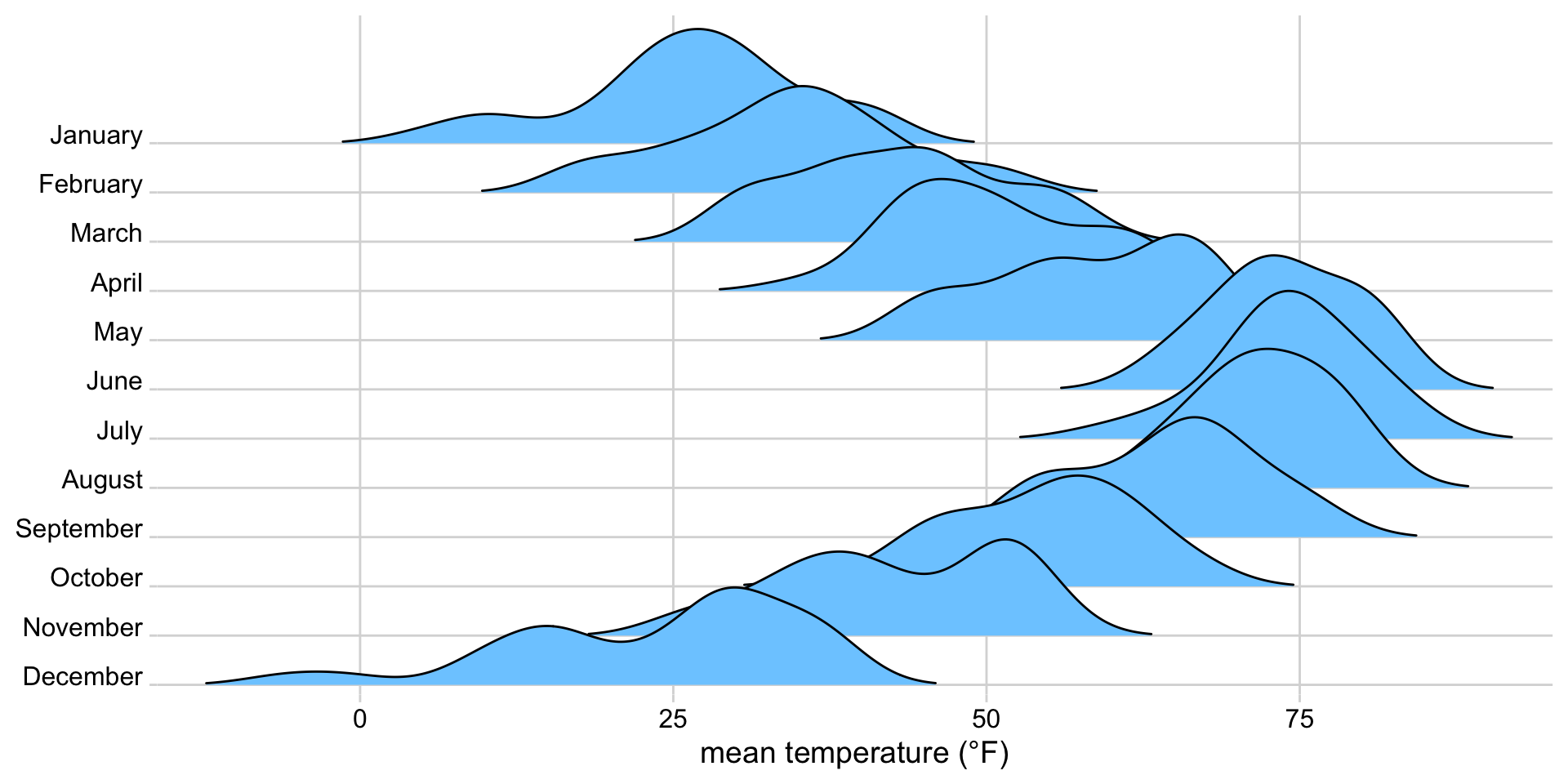
Change fill color from default gray to blue
ggplot(lincoln_temps) +
  aes(x = mean_temp, y = month_long) +
  geom_density_ridges(
    scale = 3, bandwidth = 3.4,
    rel_min_height = 0.01,
    fill = "#7DCCFF"
  ) +
  scale_x_continuous(
    name = "mean temperature (°F)",
    expand = c(0, 0)
  ) +
  scale_y_discrete(
    name = NULL,
    expand = expansion(add = c(0.2, 2.6))
  ) +
  theme_minimal_grid() +
  theme(
    axis.text.y = element_text(vjust = 0)
  )
Draw lines in white instead of black
ggplot(lincoln_temps) +
  aes(x = mean_temp, y = month_long) +
  geom_density_ridges(
    scale = 3, bandwidth = 3.4,
    rel_min_height = 0.01,
    fill = "#7DCCFF",
    color = "white"
  ) +
  scale_x_continuous(
    name = "mean temperature (°F)",
    expand = c(0, 0)
  ) +
  scale_y_discrete(
    name = NULL,
    expand = expansion(add = c(0.2, 2.6))
  ) +
  theme_minimal_grid() +
  theme(
    axis.text.y = element_text(vjust = 0)
  )
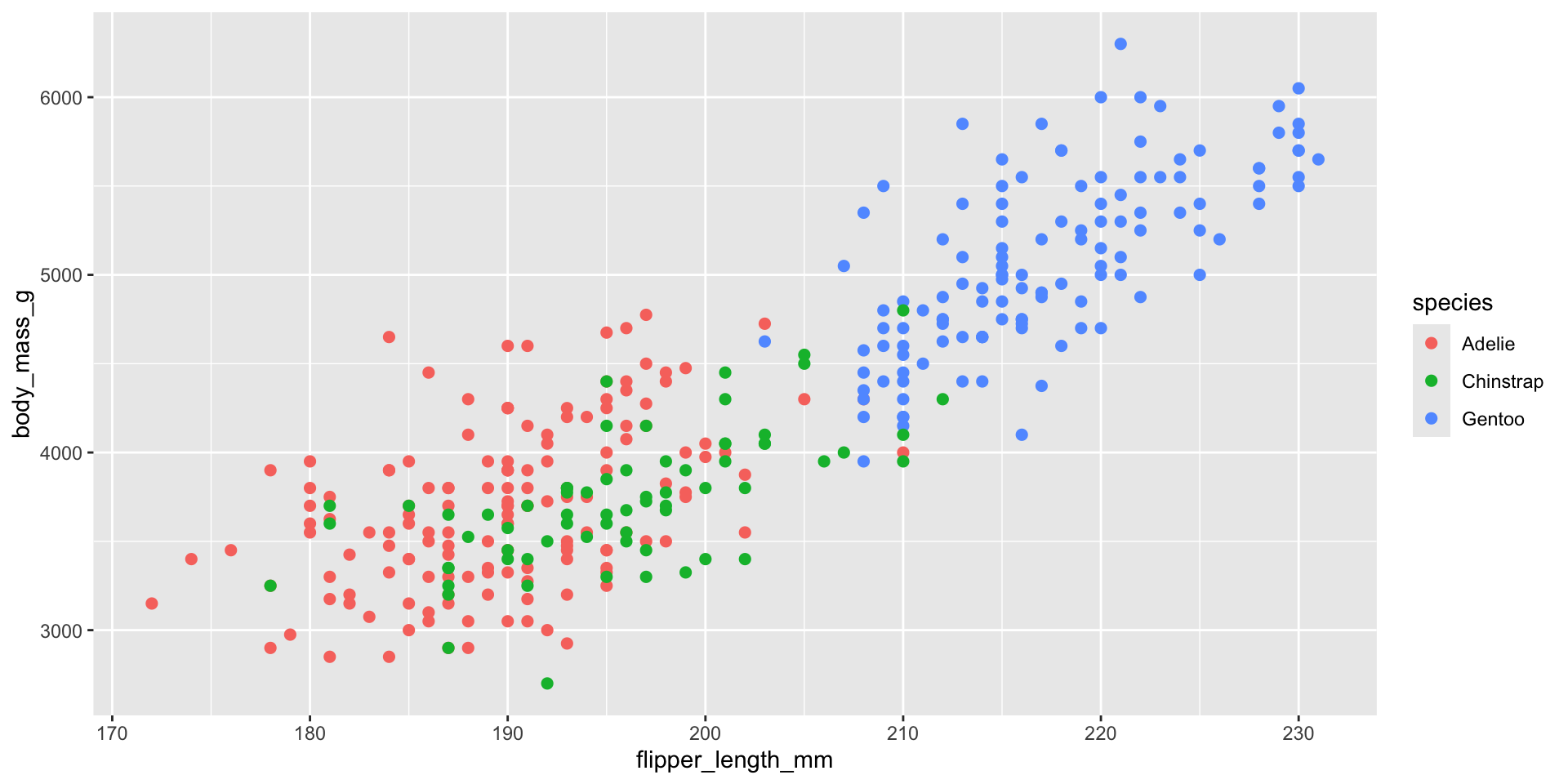
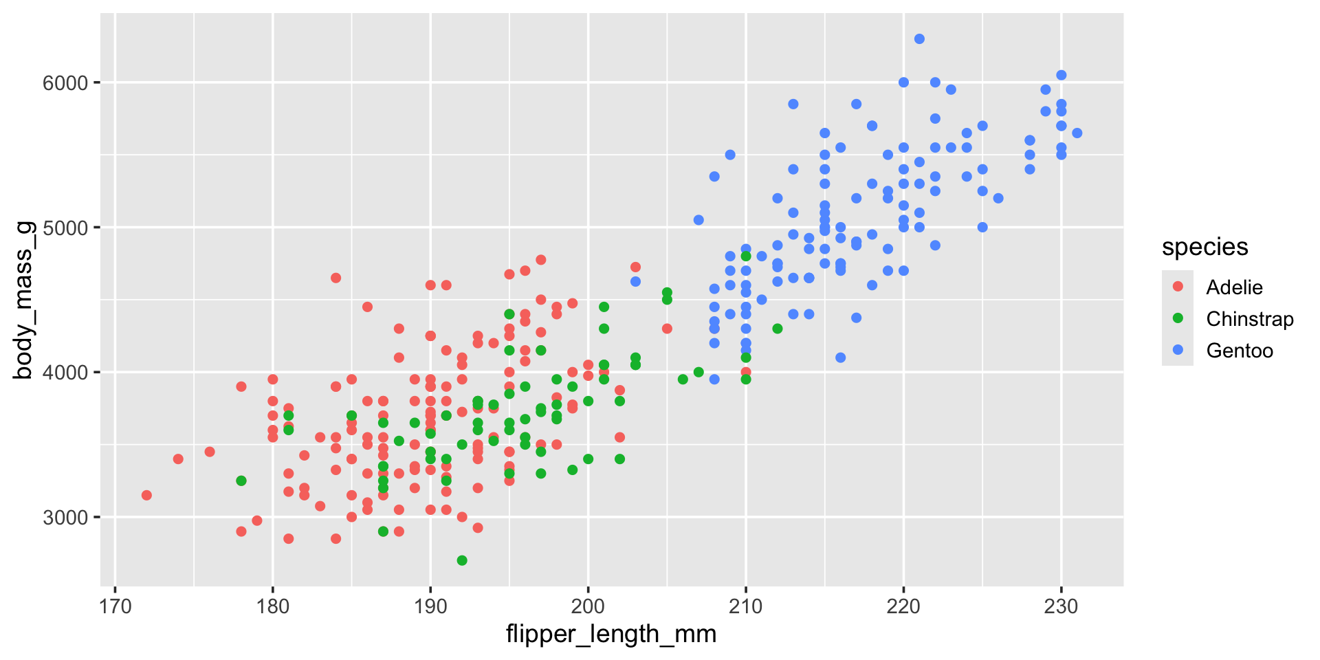
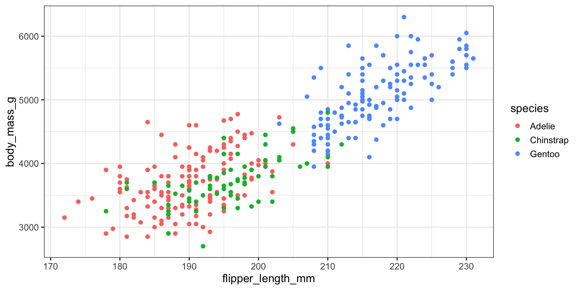
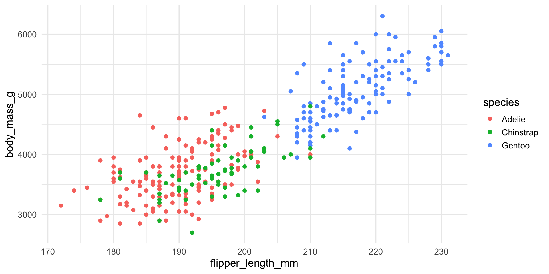
Working with ggplot themes
Using ready-made themes
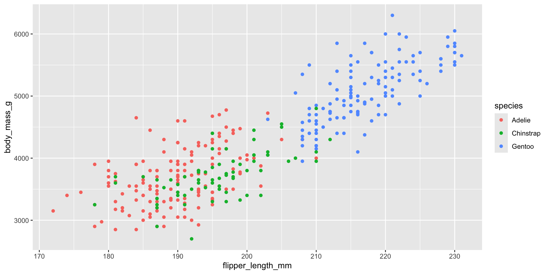
Using ready-made themes
Using ready-made themes
Using ready-made themes
Using ready-made themes
Using ready-made themes
Using ready-made themes
Using ready-made themes
Using ready-made themes
Using ready-made themes
Using ready-made themes
Using ready-made themes
Using ready-made themes
Customizing theme elements
ggplot(penguins) +
  aes(flipper_length_mm, body_mass_g) +
  geom_point(aes(color = species)) +
  theme_minimal_grid()
Customizing theme elements
ggplot(penguins) +
  aes(flipper_length_mm, body_mass_g) +
  geom_point(aes(color = species)) +
  theme_minimal_grid() +
  theme(
    # change overall font family
    # (requires font to be available)
    text = element_text(
      family = "Comic Sans MS"
    )
  )
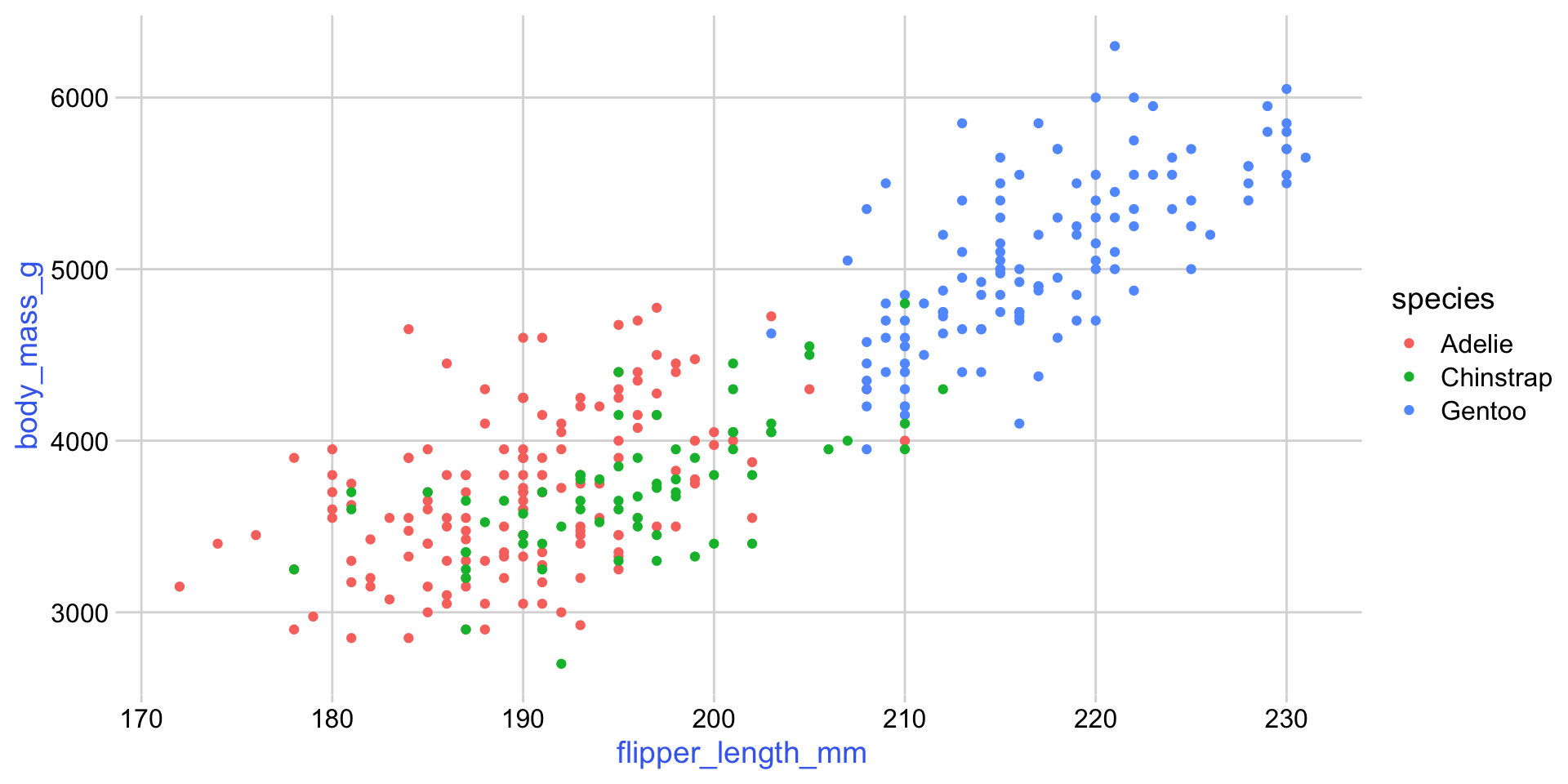
Customizing theme elements
ggplot(penguins) +
  aes(flipper_length_mm, body_mass_g) +
  geom_point(aes(color = species)) +
  theme_minimal_grid() +
  theme(
    # change color of axis titles
    axis.title = element_text(
      color = "royalblue2"
    )
  )
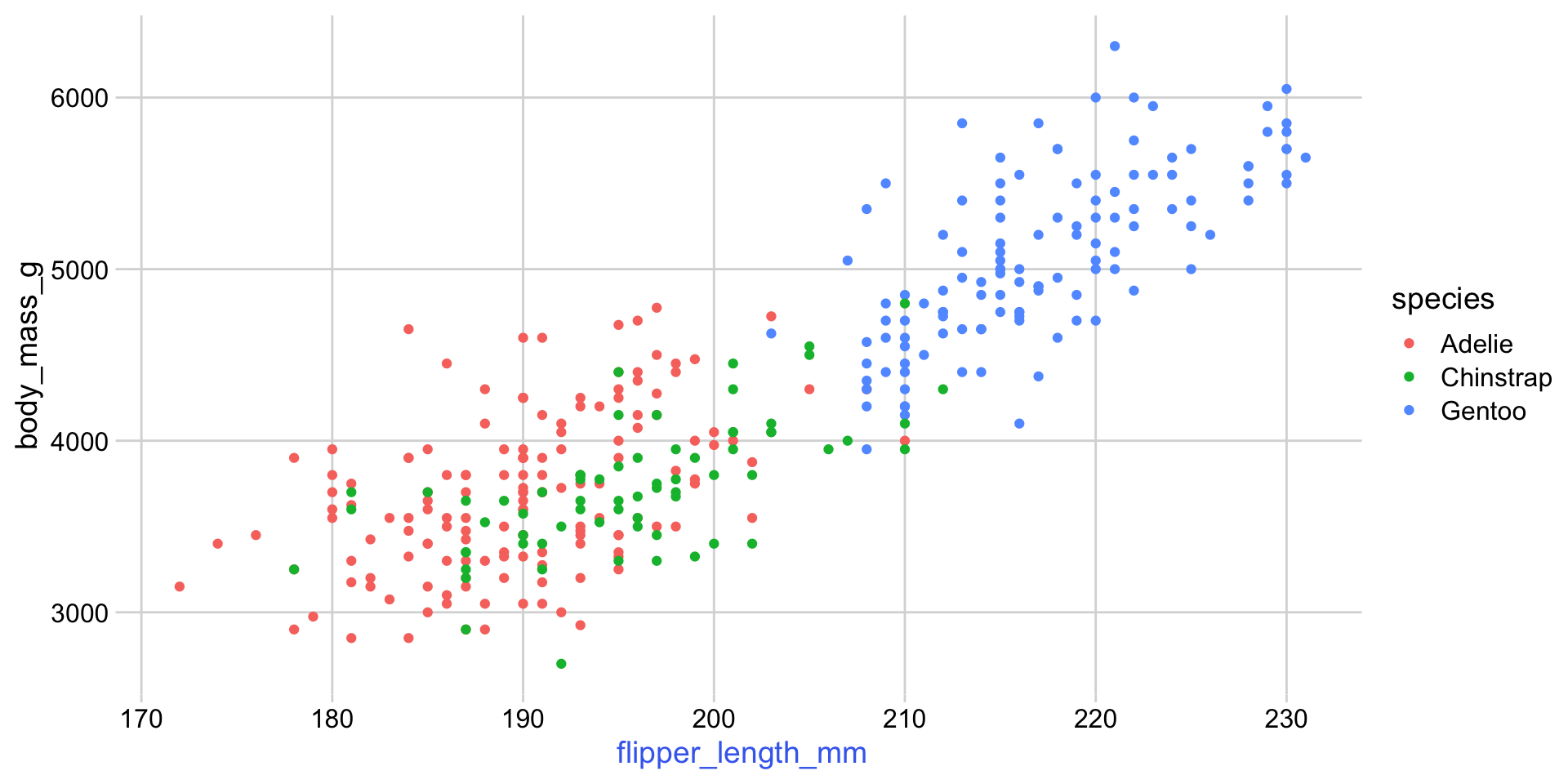
Customizing theme elements
ggplot(penguins) +
  aes(flipper_length_mm, body_mass_g) +
  geom_point(aes(color = species)) +
  theme_minimal_grid() +
  theme(
    # change color of only the x axis title
    axis.title.x = element_text(
      color = "royalblue2"
    )
  )
Customizing theme elements
ggplot(penguins) +
  aes(flipper_length_mm, body_mass_g) +
  geom_point(aes(color = species)) +
  theme_minimal_grid() +
  theme(
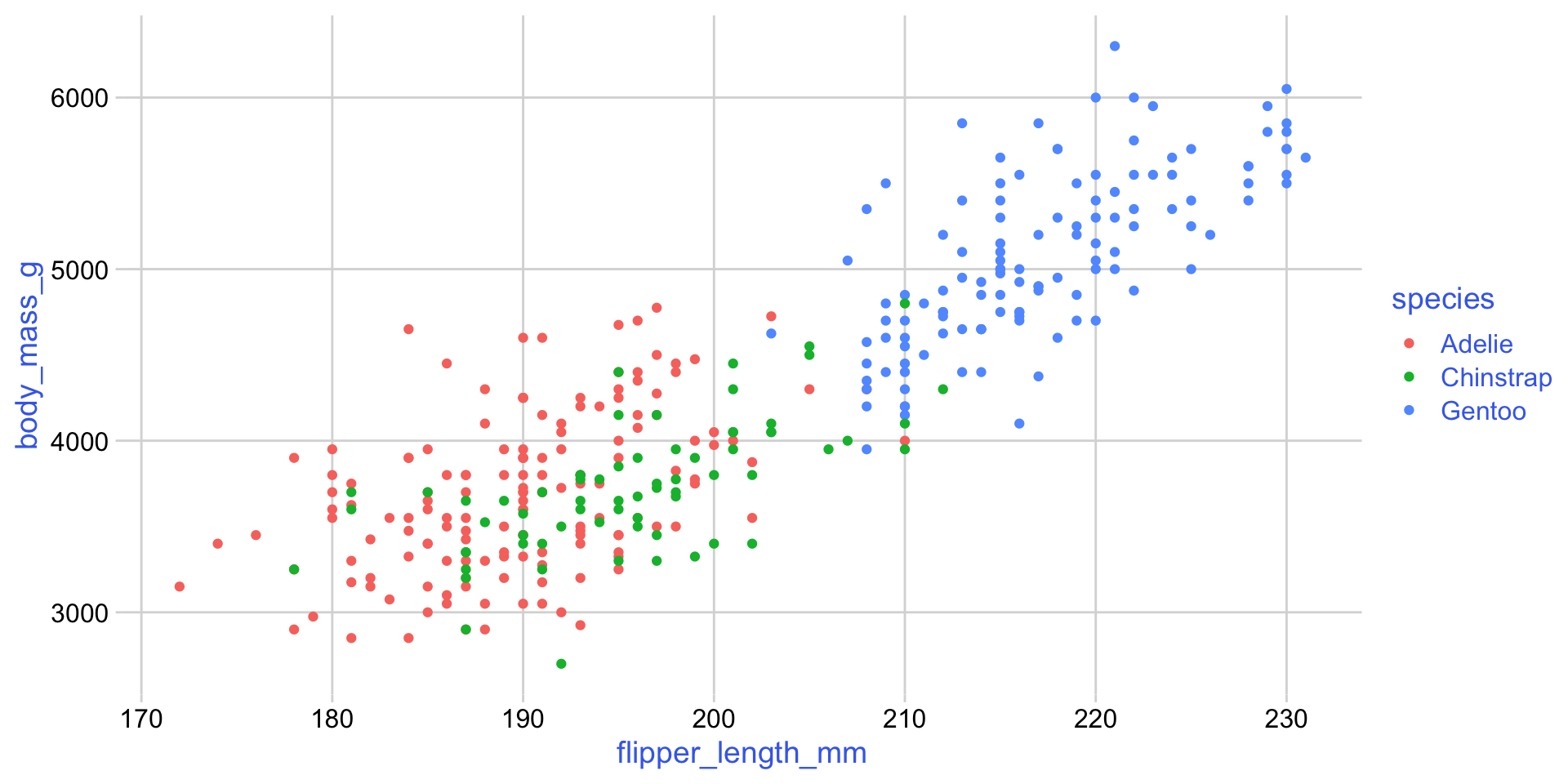
    # change all text colors?
    # why does it not work?
    text = element_text(color = "royalblue2")
  )
Customizing theme elements
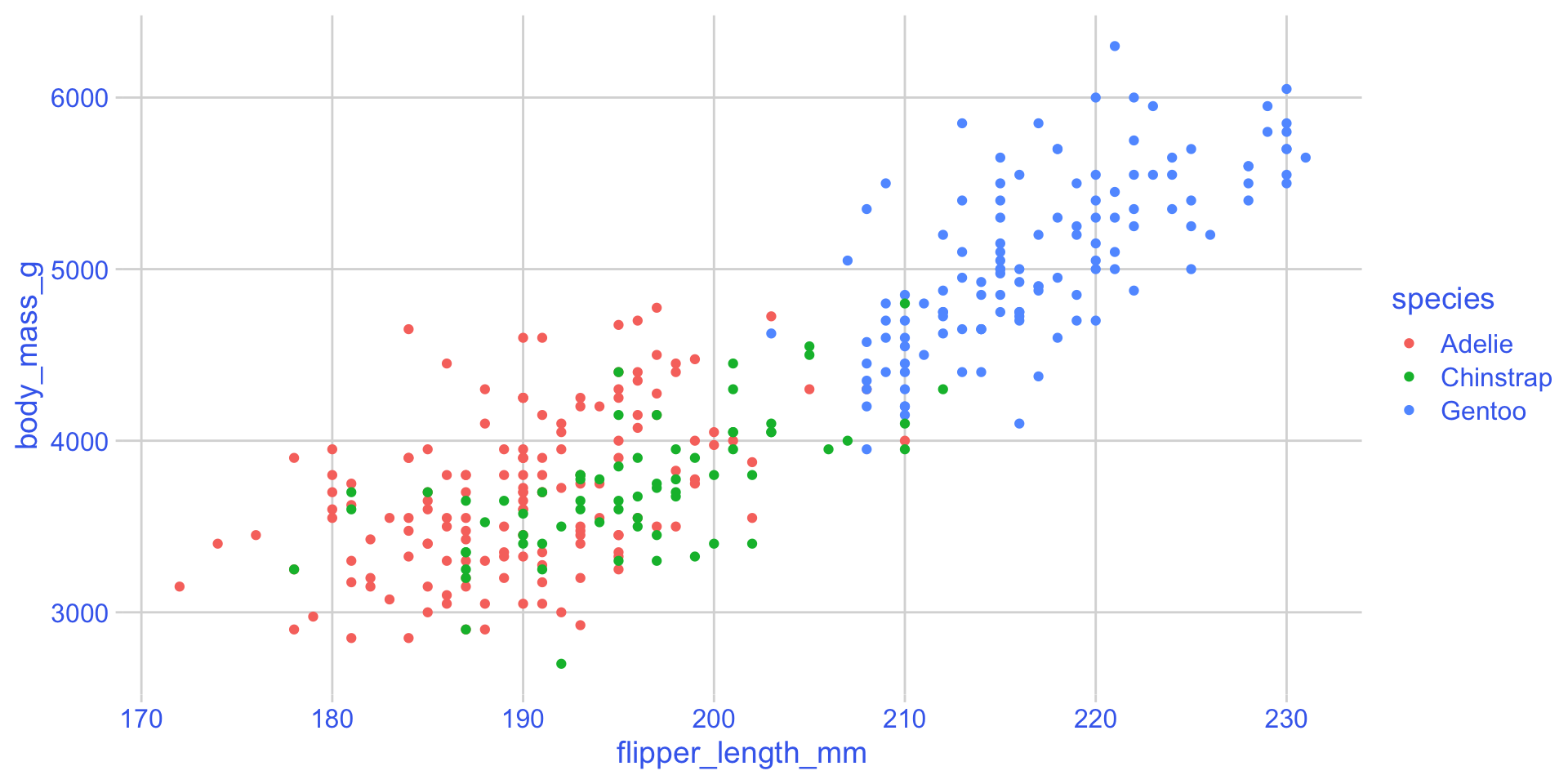
ggplot(penguins) +
  aes(flipper_length_mm, body_mass_g) +
  geom_point(aes(color = species)) +
  theme_minimal_grid() +
  theme(
    text = element_text(color = "royalblue2"),
    axis.text = element_text(
      color = "royalblue2"
    )
  )
Customizing theme elements
ggplot(penguins) +
  aes(flipper_length_mm, body_mass_g) +
  geom_point(aes(color = species)) +
  theme_minimal_grid() +
  theme(
    text = element_text(color = "royalblue2"),
    axis.text = element_text(
      color = "royalblue2"
    )
  )
The element axis.text has its own color set in the theme. Therefore it doesn’t inherit from text.
Horizontal and vertical alignment
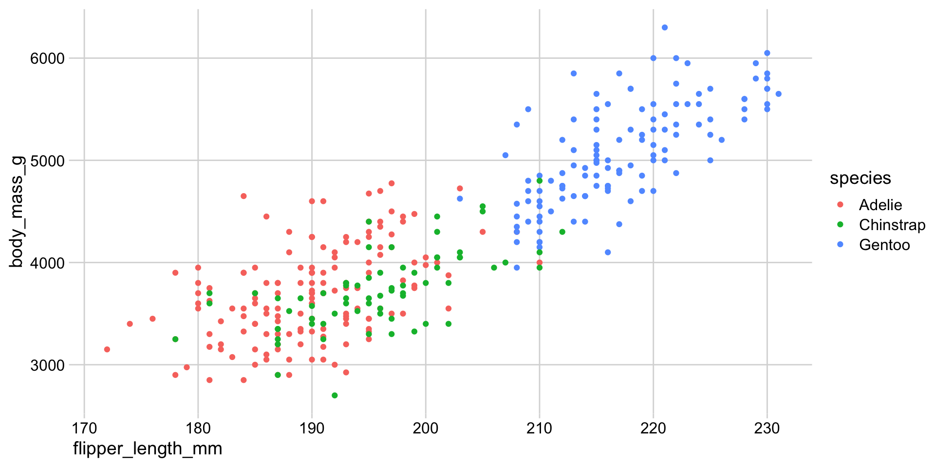
ggplot(penguins) +
  aes(flipper_length_mm, body_mass_g) +
  geom_point(aes(color = species)) +
  theme_minimal_grid() +
  theme(
    axis.title.x = element_text(
      # horizontal justification
      # (0 = left)
      hjust = 0
    )
  )
Horizontal and vertical alignment
ggplot(penguins) +
  aes(flipper_length_mm, body_mass_g) +
  geom_point(aes(color = species)) +
  theme_minimal_grid() +
  theme(
    axis.title.x = element_text(
      # horizontal justification
      # (0.5 = center)
      hjust = 0.5
    )
  )
Horizontal and vertical alignment
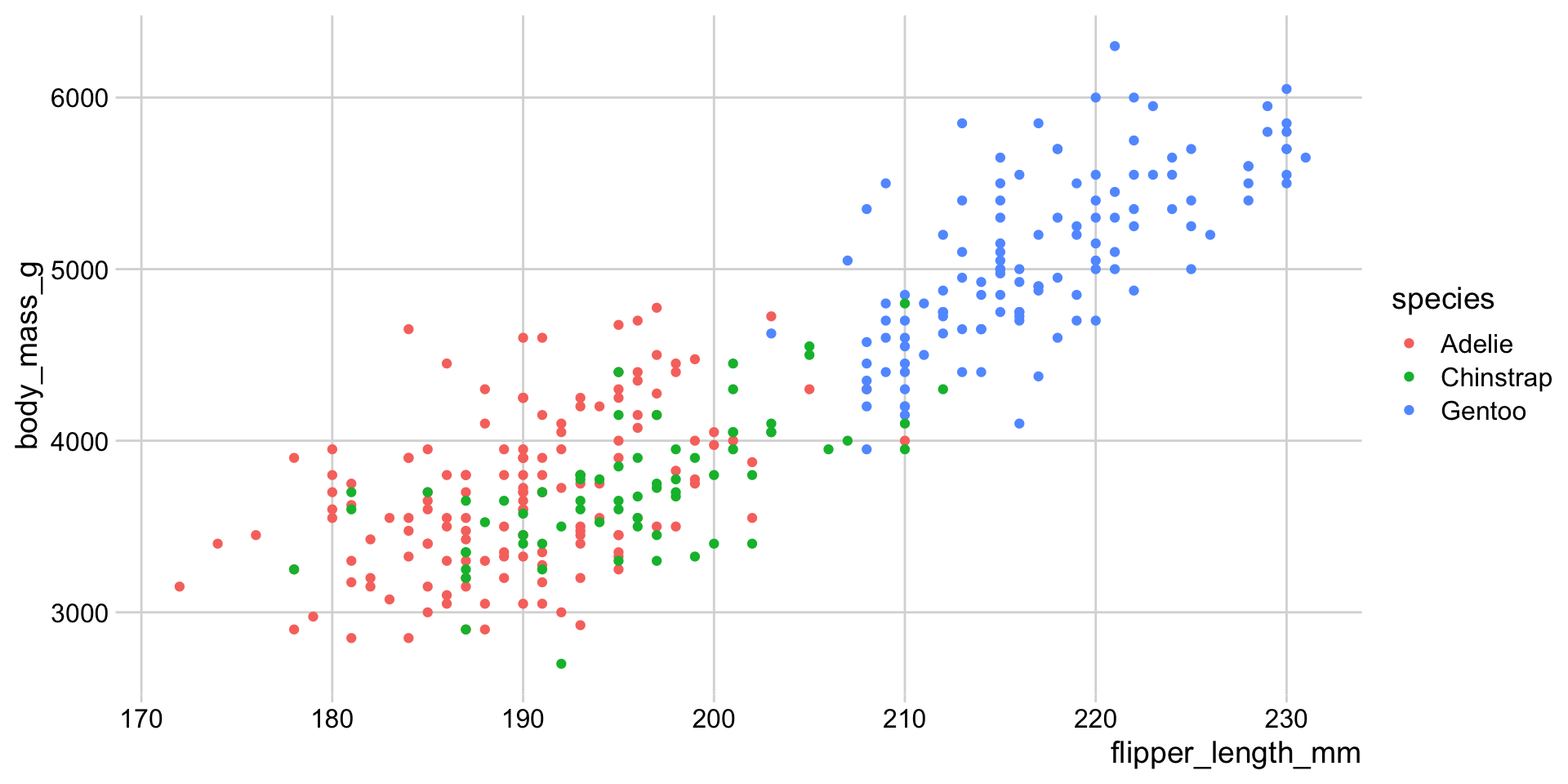
ggplot(penguins) +
  aes(flipper_length_mm, body_mass_g) +
  geom_point(aes(color = species)) +
  theme_minimal_grid() +
  theme(
    axis.title.x = element_text(
      # horizontal justification
      # (1 = right)
      hjust = 1
    )
  )
Horizontal and vertical alignment
ggplot(penguins) +
  aes(flipper_length_mm, body_mass_g) +
  geom_point(aes(color = species)) +
  theme_minimal_grid() +
  theme(
    axis.text.y = element_text(
      # vertical justification
      # (0 = bottom)
      vjust = 0
    )
  )
Horizontal and vertical alignment
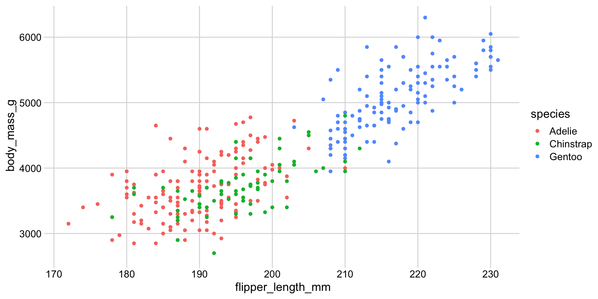
ggplot(penguins) +
  aes(flipper_length_mm, body_mass_g) +
  geom_point(aes(color = species)) +
  theme_minimal_grid() +
  theme(
    axis.text.y = element_text(
      # vertical justification
      # (0.5 = center)
      vjust = 0.5
    )
  )
Horizontal and vertical alignment
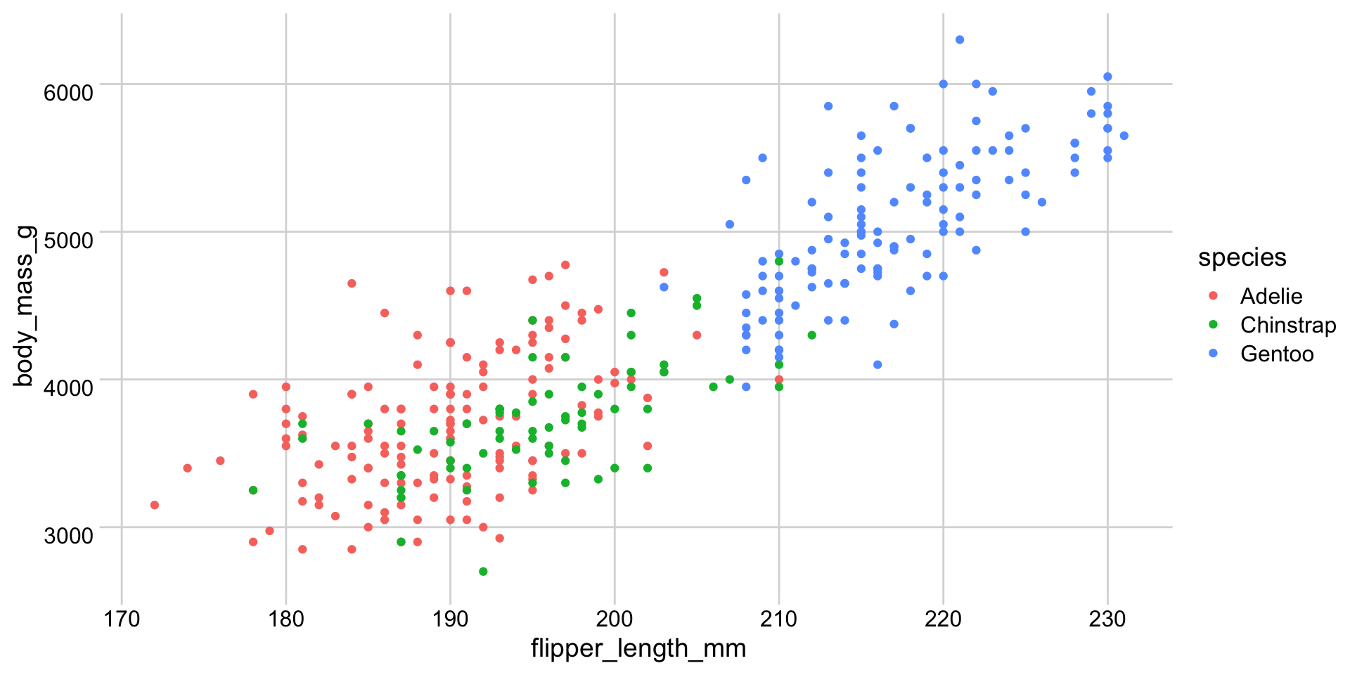
ggplot(penguins) +
  aes(flipper_length_mm, body_mass_g) +
  geom_point(aes(color = species)) +
  theme_minimal_grid() +
  theme(
    axis.text.y = element_text(
      # vertical justification
      # (1 = top)
      vjust = 1
    )
  )
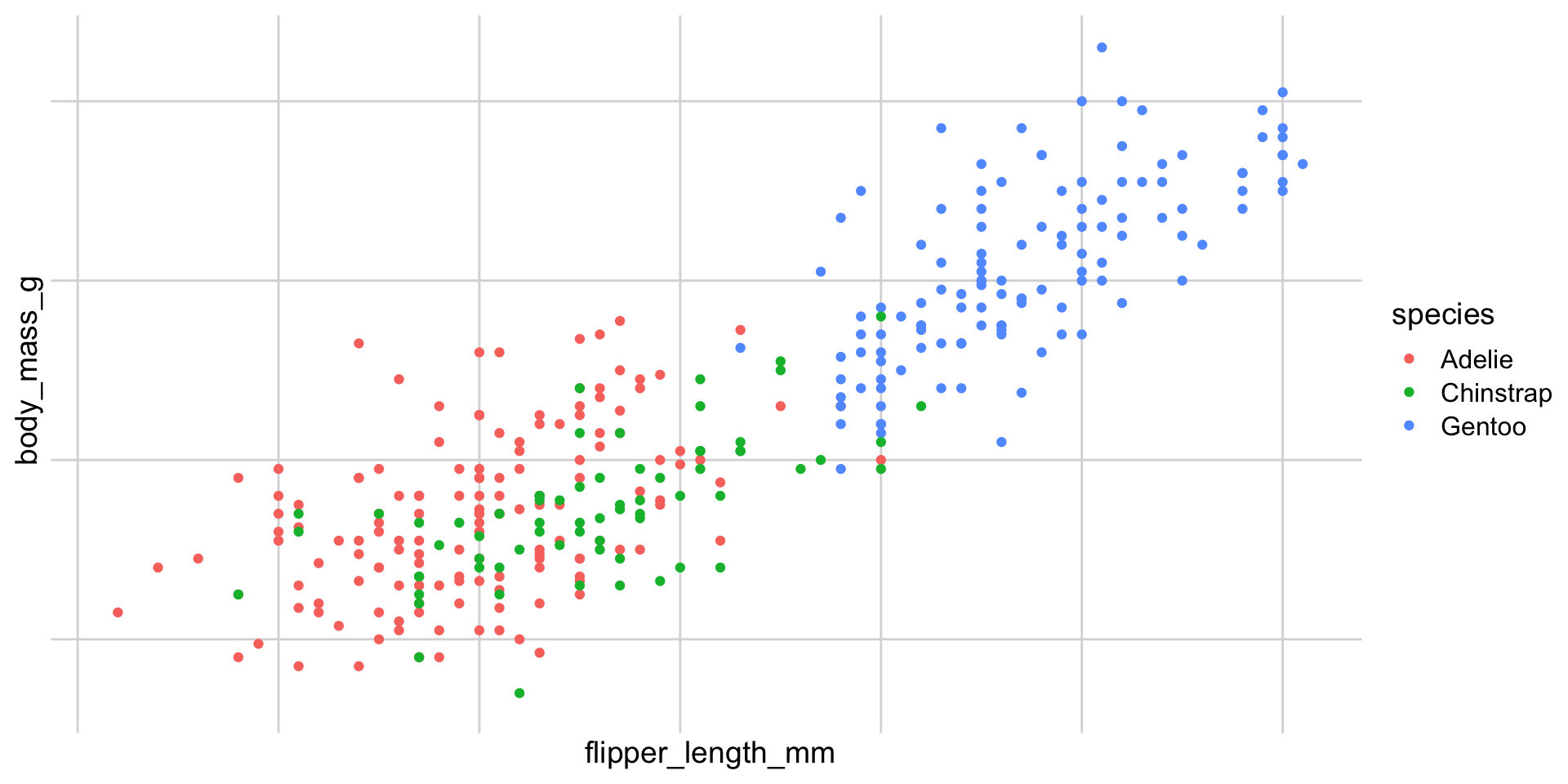
Remove elements entirely: element_blank()
ggplot(penguins) +
  aes(flipper_length_mm, body_mass_g) +
  geom_point(aes(color = species)) +
  theme_minimal_grid() +
  theme(
    # all text gone
    axis.text = element_blank()
  )
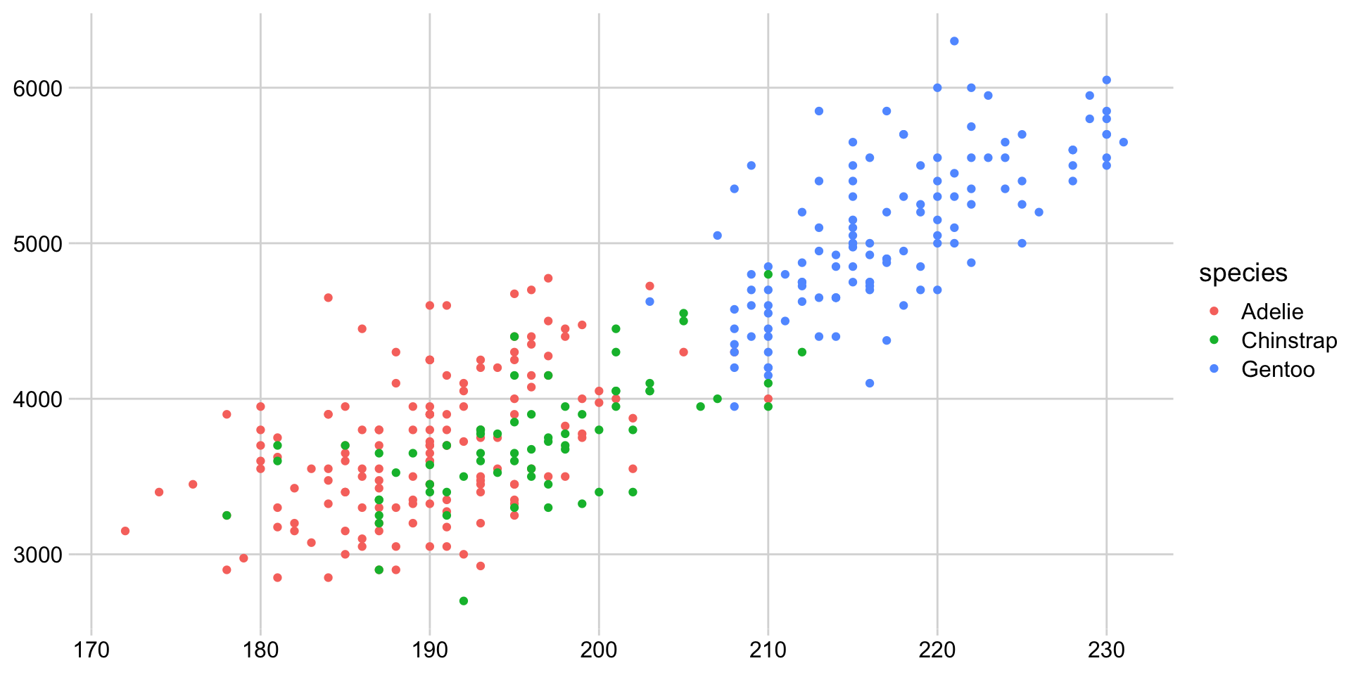
Remove elements entirely: element_blank()
ggplot(penguins) +
  aes(flipper_length_mm, body_mass_g) +
  geom_point(aes(color = species)) +
  theme_minimal_grid() +
  theme(
    # no axis titles
    axis.title = element_blank()
  )
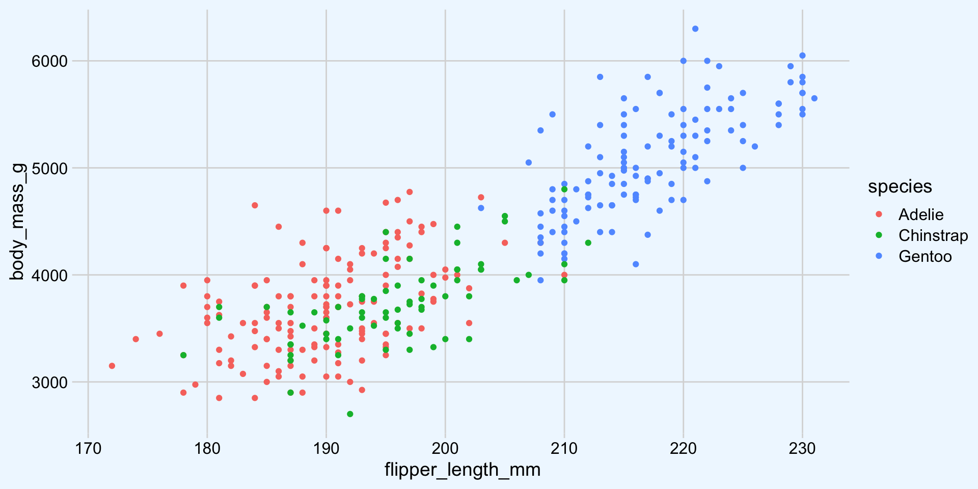
Set background color: element_rect()
ggplot(penguins) +
  aes(flipper_length_mm, body_mass_g) +
  geom_point(aes(color = species)) +
  theme_minimal_grid() +
  theme(
    plot.background = element_rect(
      fill = "aliceblue"
    )
  )
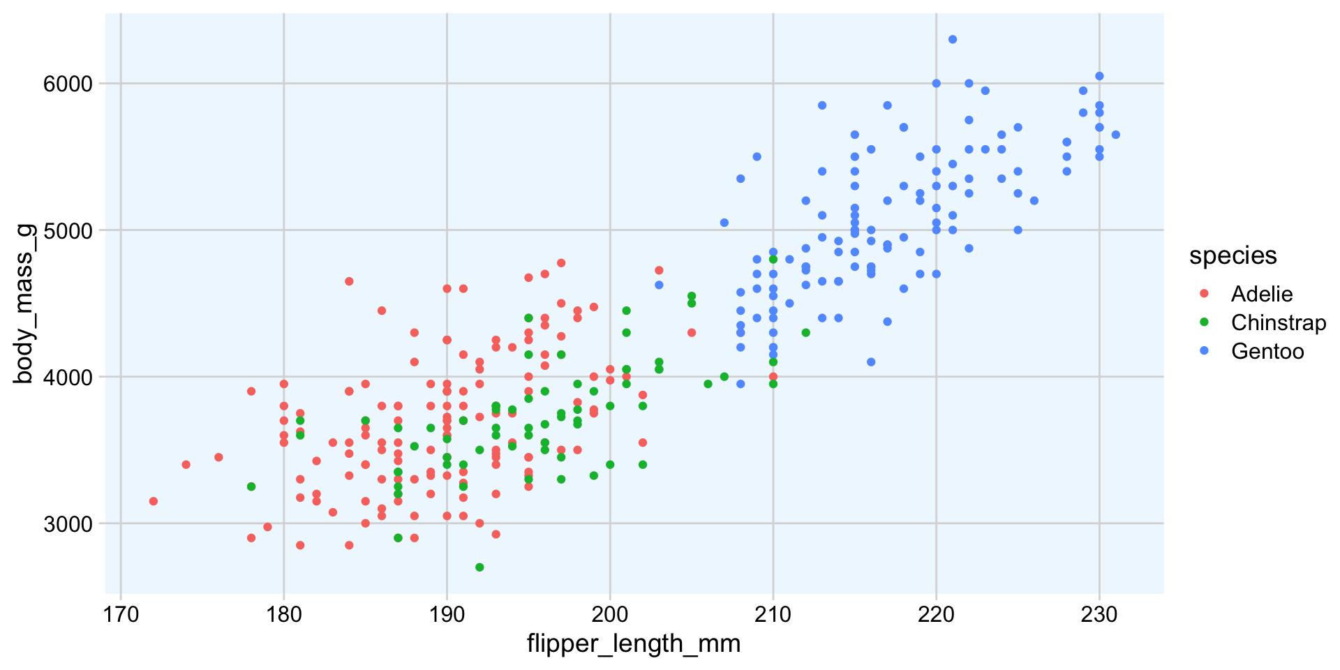
Set background color: element_rect()
ggplot(penguins) +
  aes(flipper_length_mm, body_mass_g) +
  geom_point(aes(color = species)) +
  theme_minimal_grid() +
  theme(
    panel.background = element_rect(
      fill = "aliceblue"
    )
  )
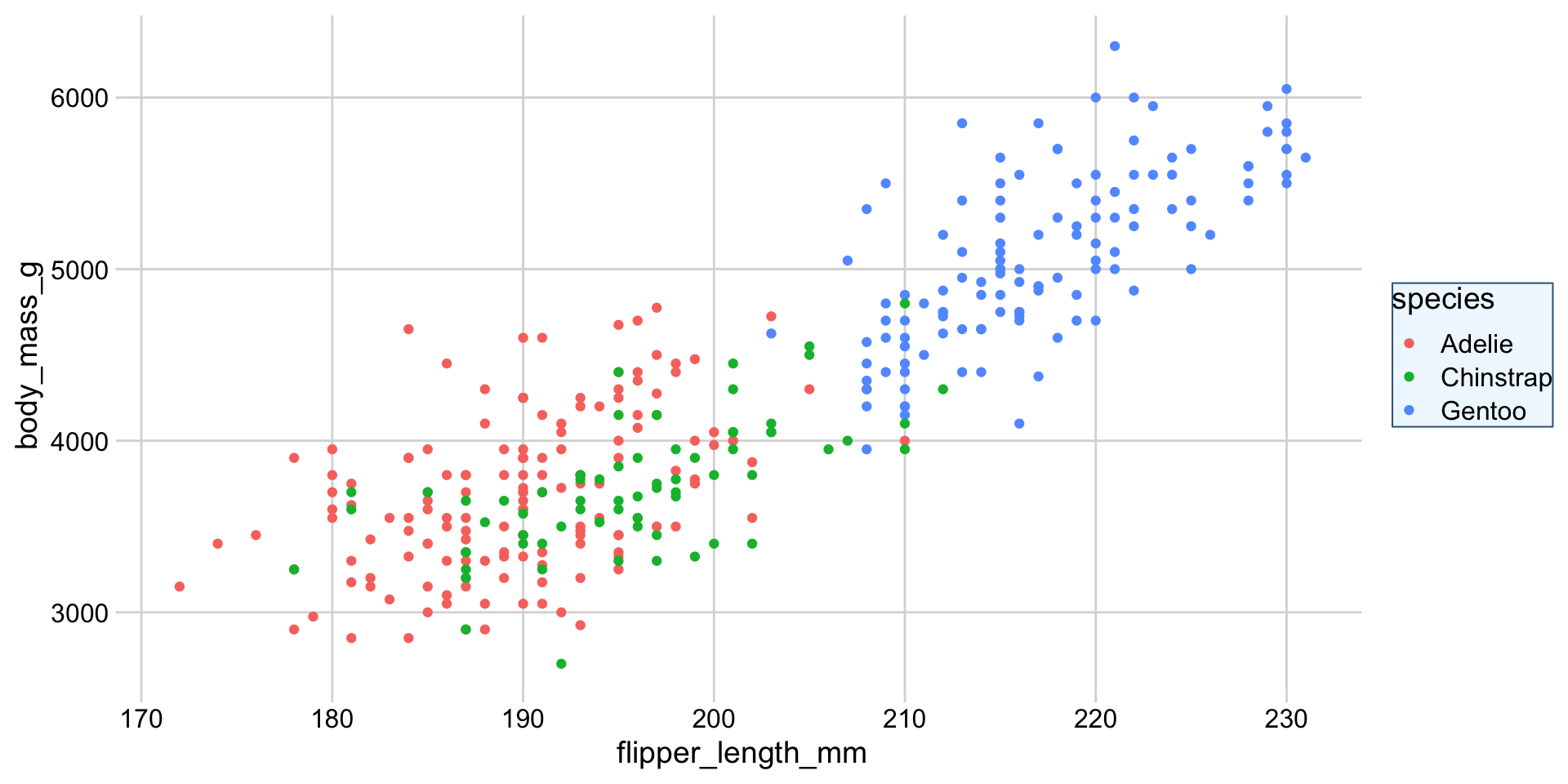
Set background color: element_rect()
ggplot(penguins) +
  aes(flipper_length_mm, body_mass_g) +
  geom_point(aes(color = species)) +
  theme_minimal_grid() +
  theme(
    legend.box.background = element_rect(
      fill = "aliceblue",
      color = "steelblue4" # line color
    )
  )
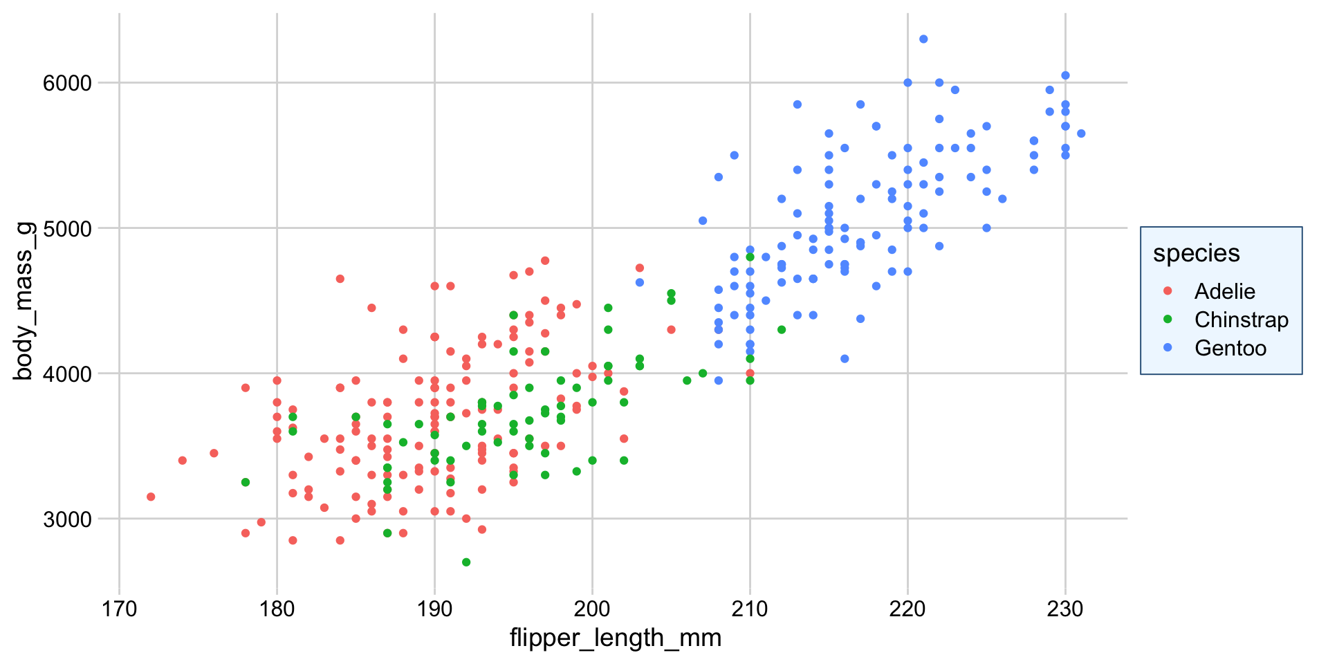
Set background color: element_rect()
ggplot(penguins) +
  aes(flipper_length_mm, body_mass_g) +
  geom_point(aes(color = species)) +
  theme_minimal_grid() +
  theme(
    legend.box.background = element_rect(
      fill = "aliceblue",
      color = "steelblue4" # line color
    ),
    legend.box.margin = margin(7, 7, 7, 7)
  )
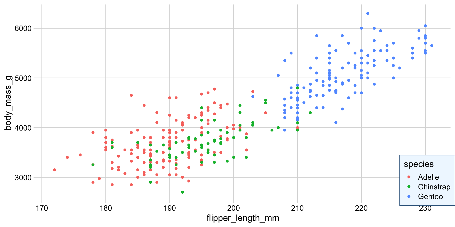
Move the legend: legend.position
ggplot(penguins) +
  aes(flipper_length_mm, body_mass_g) +
  geom_point(aes(color = species)) +
  theme_minimal_grid() +
  theme(
    legend.box.background = element_rect(
      fill = "aliceblue",
      color = "steelblue4" # line color
    ),
    legend.box.margin = margin(7, 7, 7, 7),
    # relative position inside plot panel
    legend.position = c(1, 0),
    # justification relative to position
    legend.justification = c(1, 0)
  )
Exercise
Go to https://elsherbini.github.io/durban-data-science-for-biology/materials/1-workshop1/7-custom-data-visualizations/#coding-exercise-7.2 and complete the Compound Figures exercise.
