[1] FALSEIntro to R,R Studio, and Quarto
remixed from Claus O. Wilke’s SDS375 course and Andrew P. Bray’s quarto workshop
Workshop materials are at:
https://elsherbini.github.io/durban-data-science-for-biology/
Goals for this session
Answer the question “Why R?”
Learn how to use Quarto to make notebook reports.
Begin interacting with data in R.
Discussions: discord
Ask questions at #workshop-questions on https://discord.gg/UDAsYTzZE.
Stickies
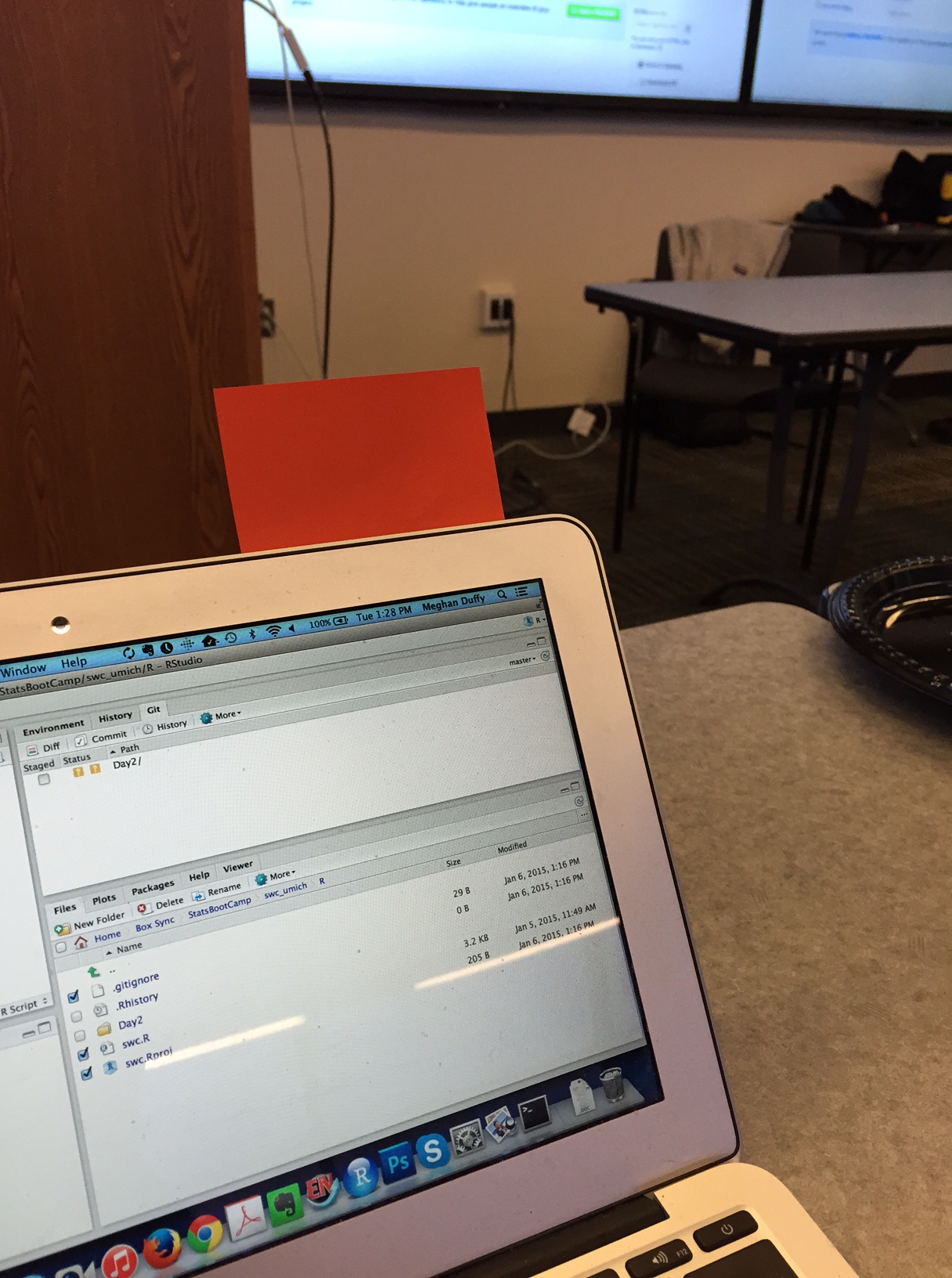
During an activity, place a blue sticky on your laptop if you’re good to go and a pink sticky if you want help.
Image by Megan Duffy
Practicalities
WiFi:
Network: KTB Free Wifi (no password needed)
Network AHRI Password: @hR1W1F1!17
Network CAPRISA-Corp Password: corp@caprisa17
Bathrooms are out the lobby to your left
What is R?
R is a general purpose programming language that’s really well suited to statistics, manipulating tabular data, and plotting.
Why R?
Why R?
- R is completely free and open source
- Using R connects you with a community around the whole world
- R has a huge amount of packages - code someone else wrote so you don’t have to!
Obtaining R
Windows, Mac or Linux OS: https://www.r-project.org
Running R
RStudio
- RStudio: http://www.rstudio.com
- Built-in tools for viewing plots, tables, and rendering documents
- The best way to work if you only use R
VSCode
- https://code.visualstudio.com/download
- not a full IDE, but you can customize it with extensions
- Works well with not just R, but all major programming languages
- Guide on setting up VSCode for R programming: link and link
Create an R Project
- File -> New Project…
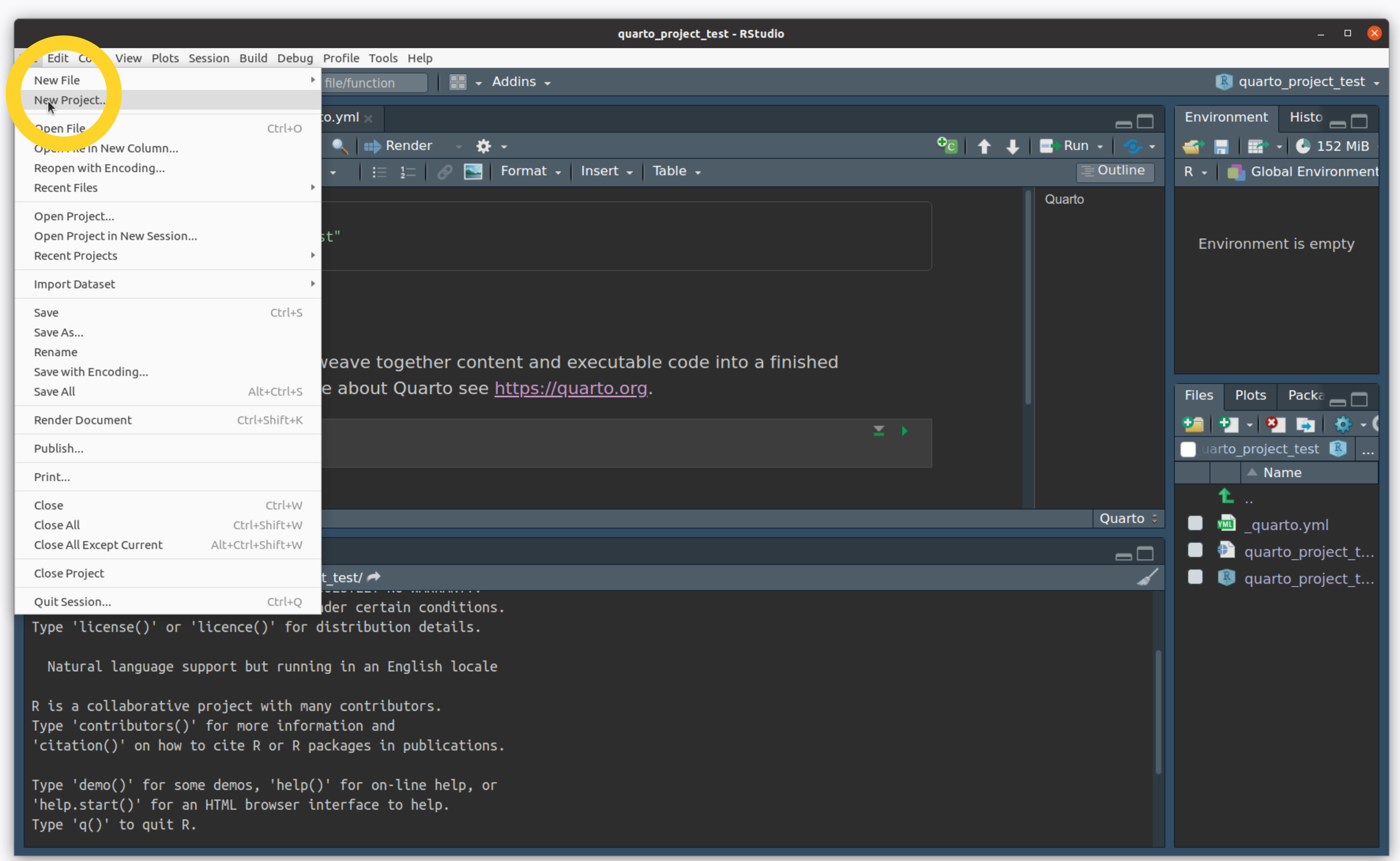
Create an R Project
- Click on New Directory
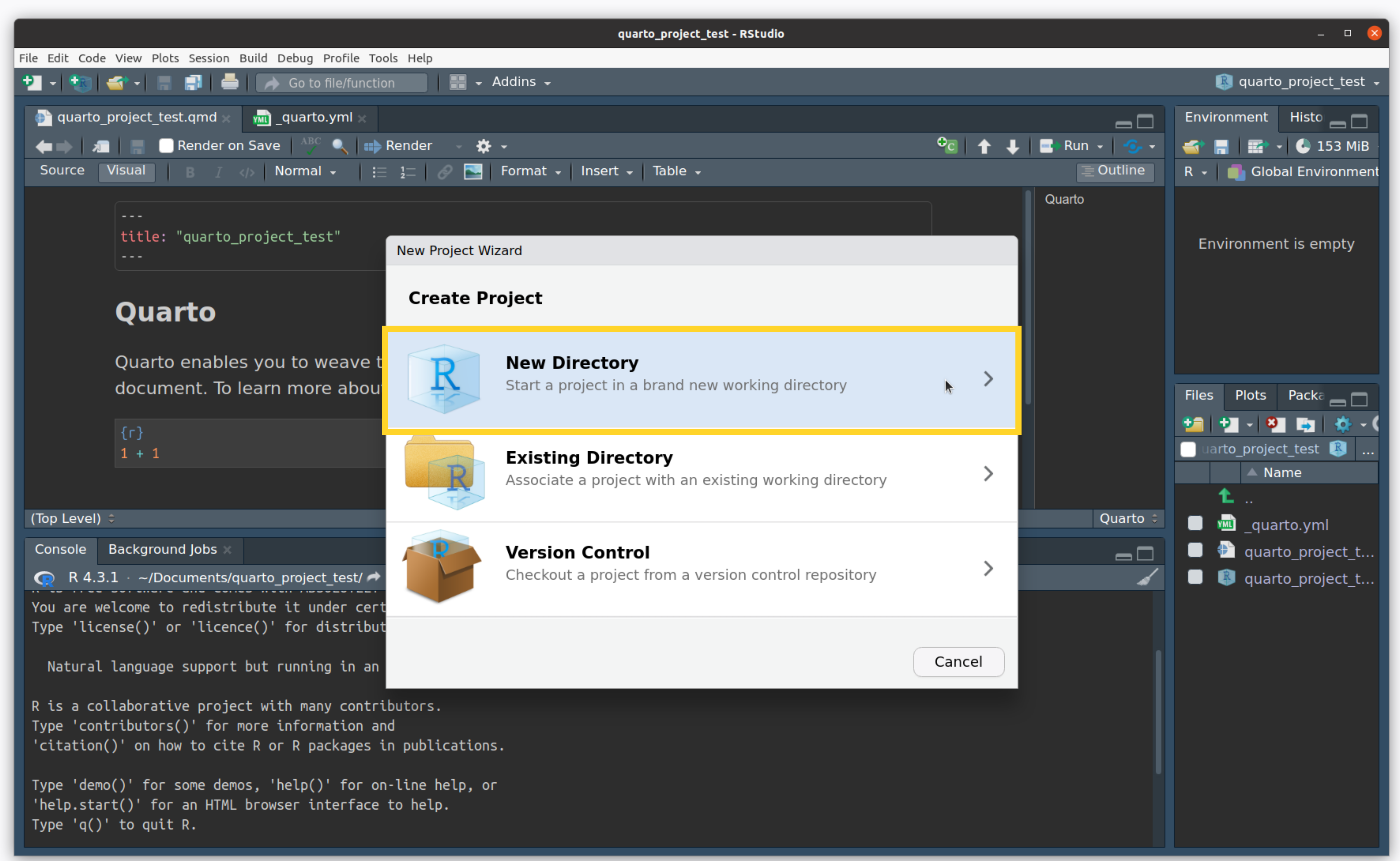
Create an R Project
- Name your directory and click “Create Project”
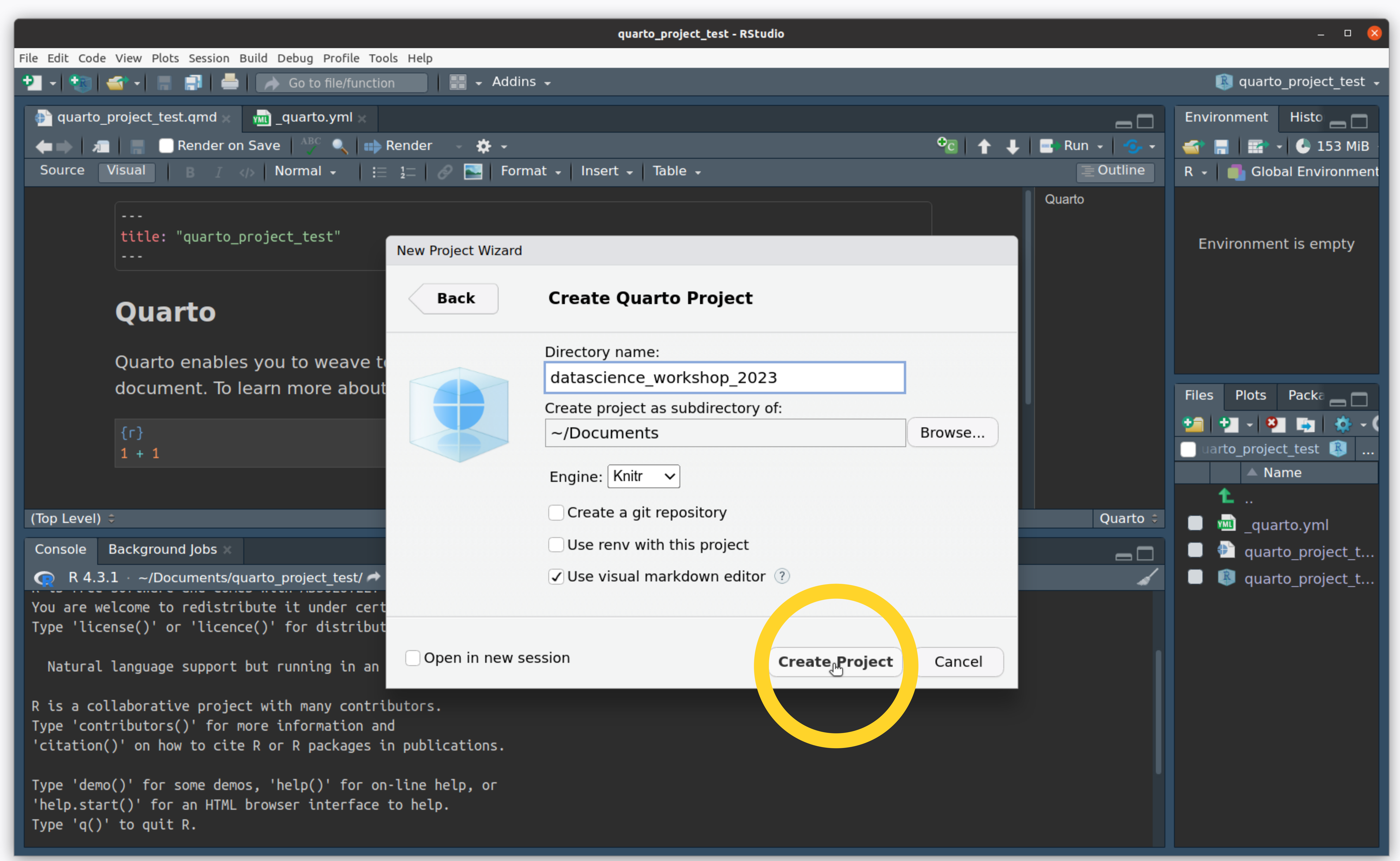
Create an R Project
- You made a project! This creates a file for you with the
.qmdextension
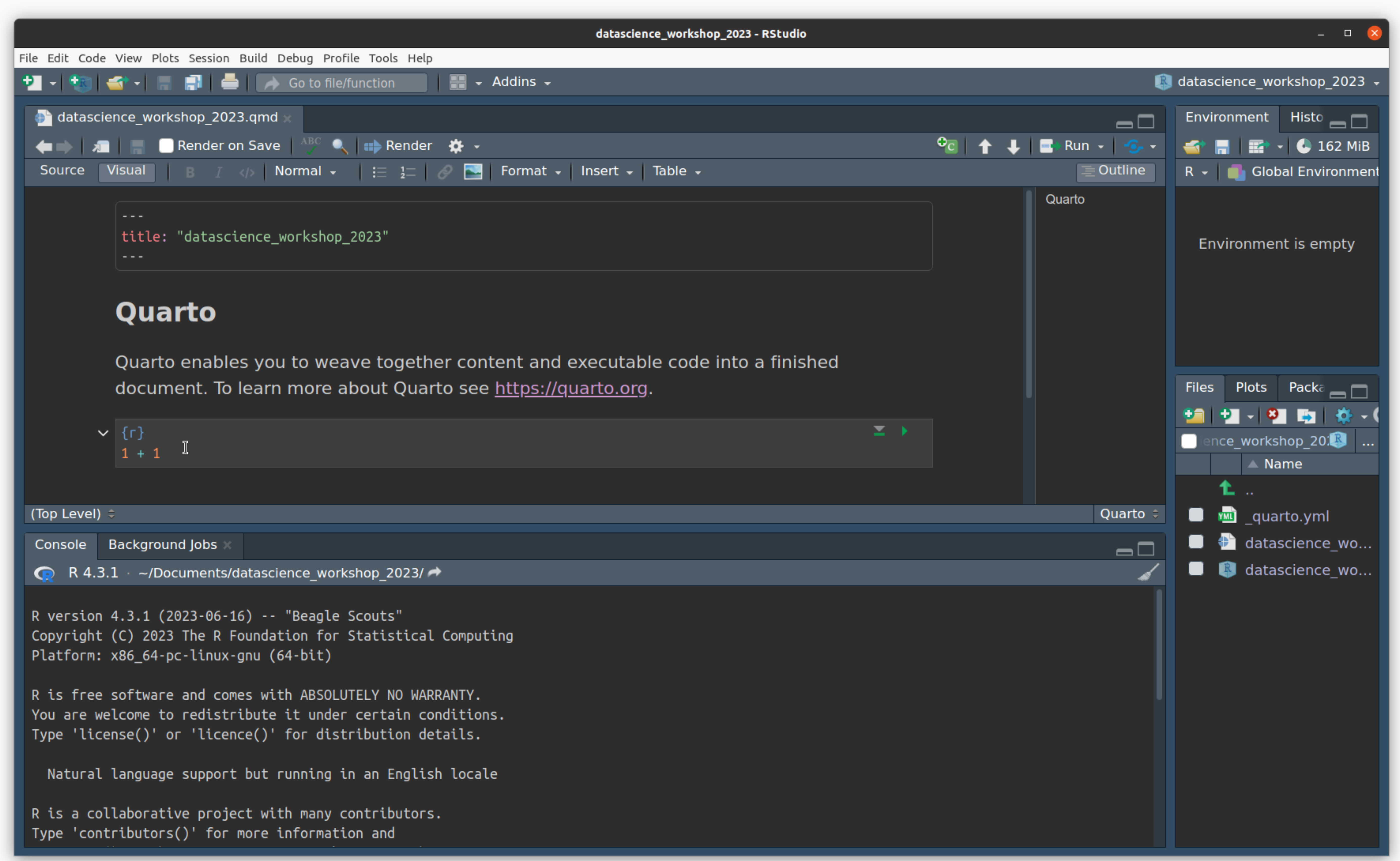
Create an R Project
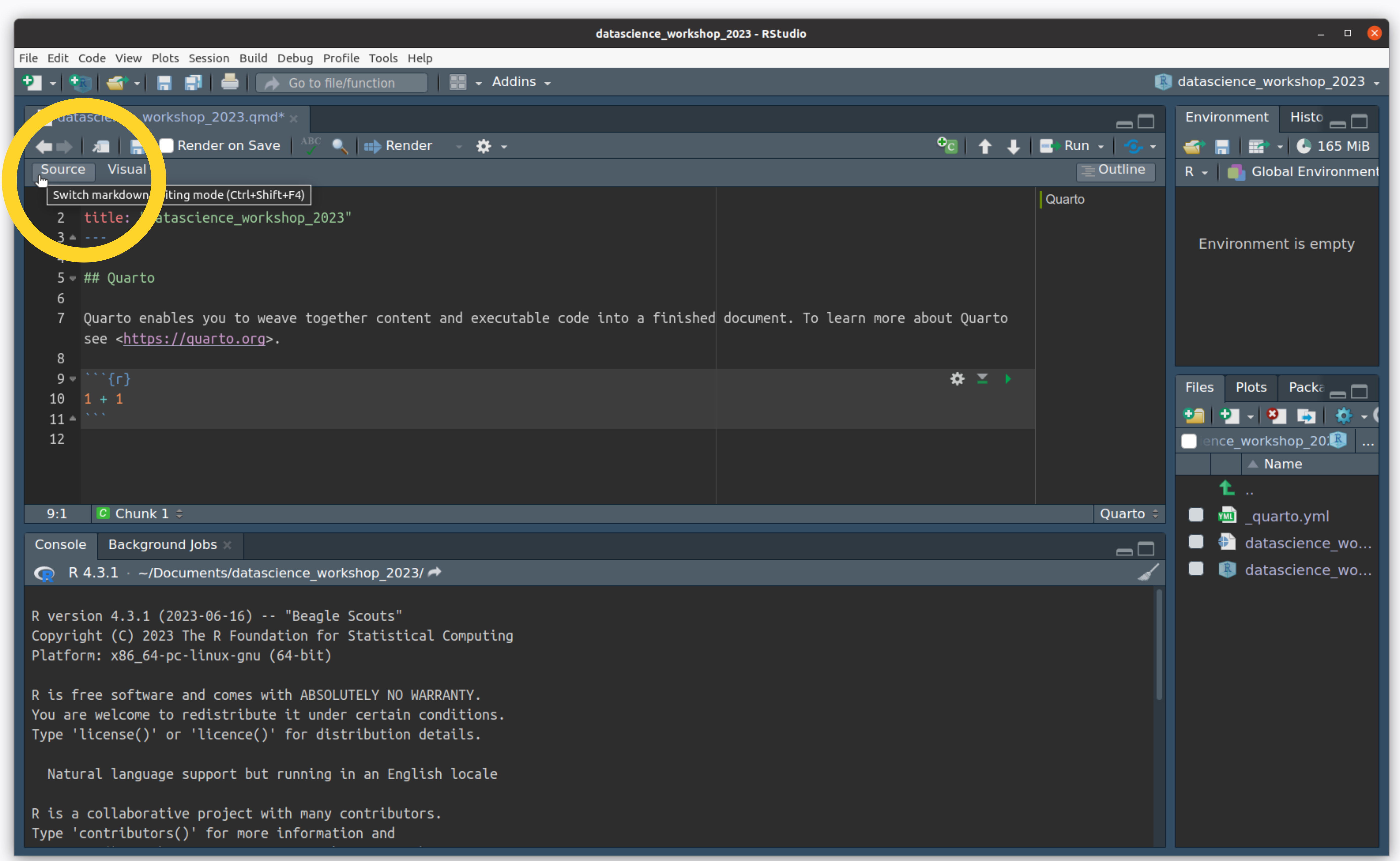
- Switch from “visual” to “source” to see the plain-text version of this document.
Create an R Project
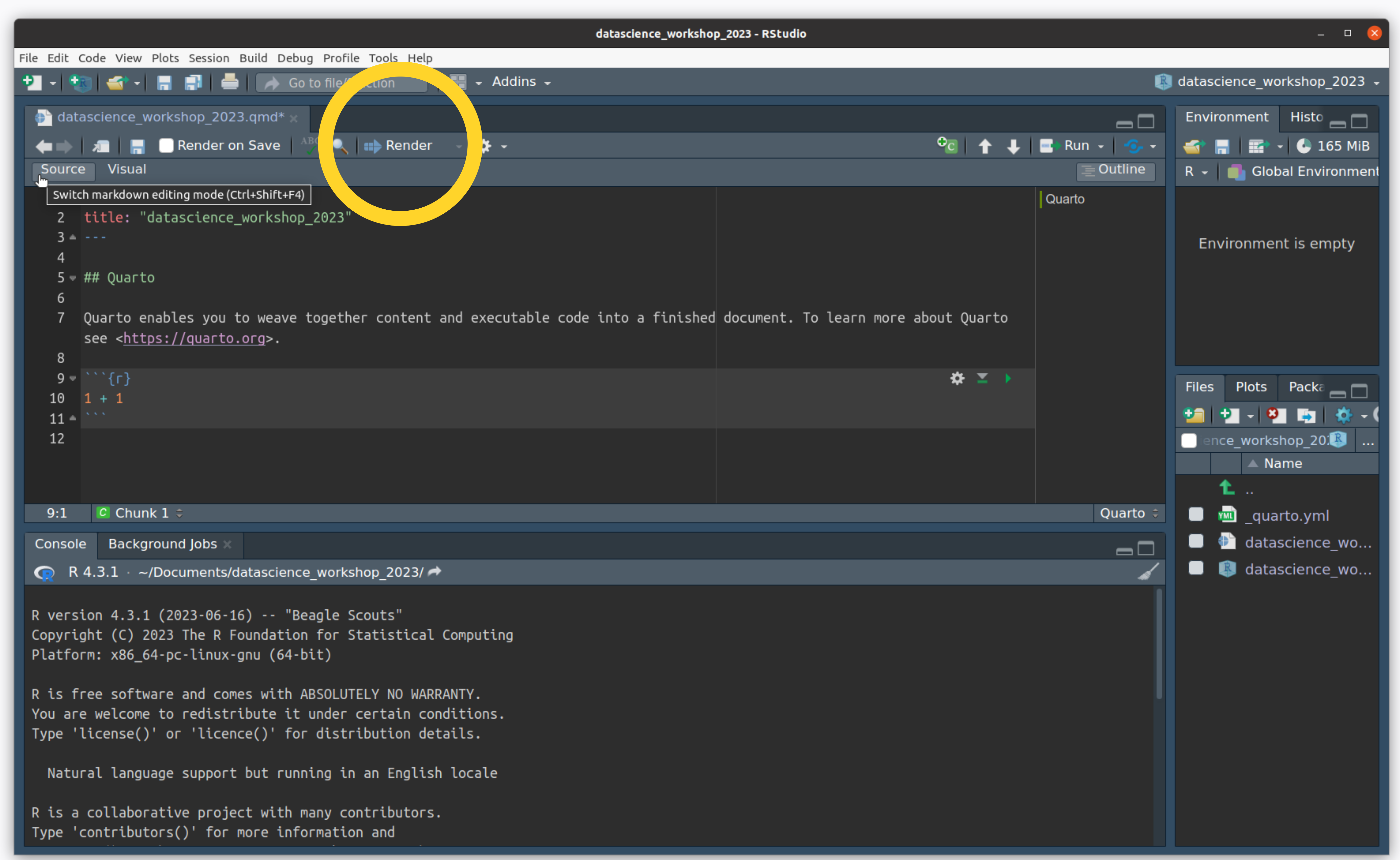
- Click on “Render” to ask Quarto to turn this plain-text document into an HTML page
Create an R Project
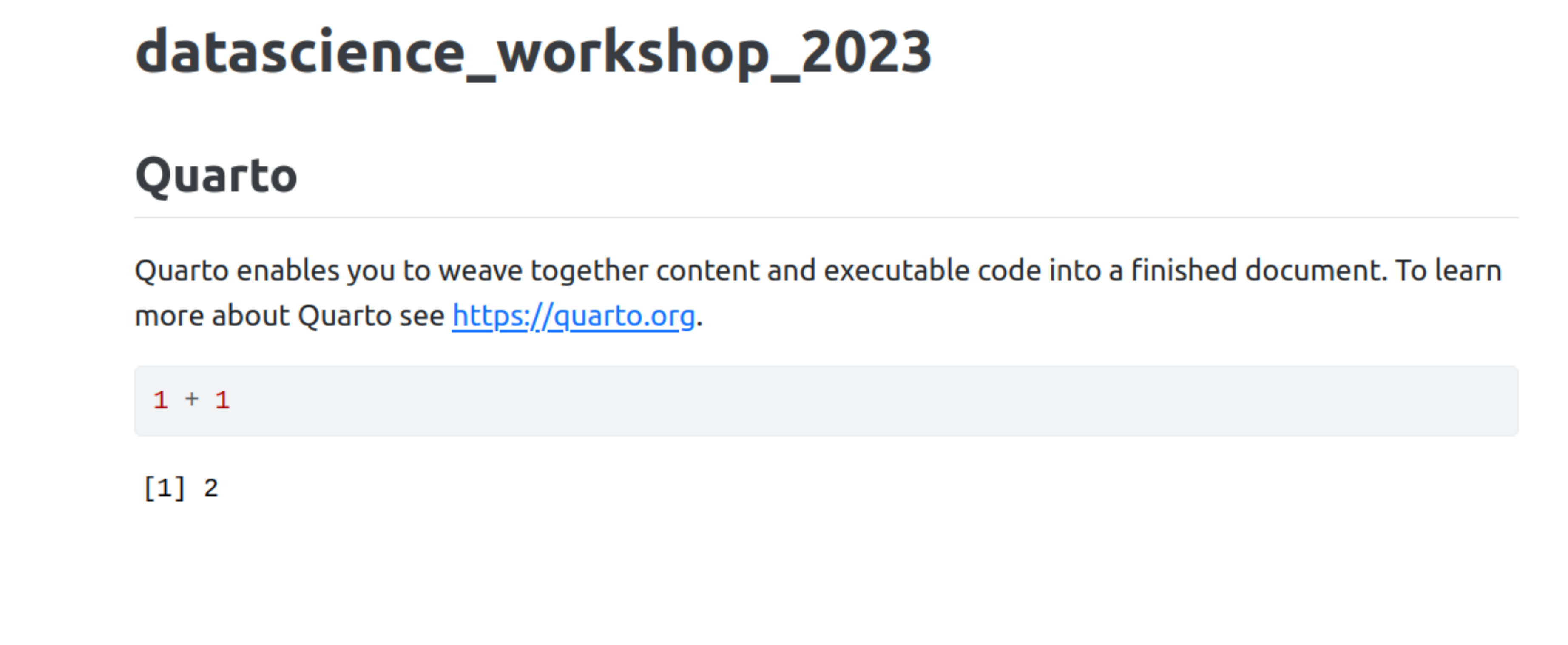
- Your default web-browser will open and show you the rendered document!
RStudio
What are the parts of RStudio?
The text editor
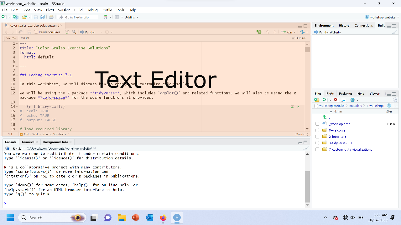
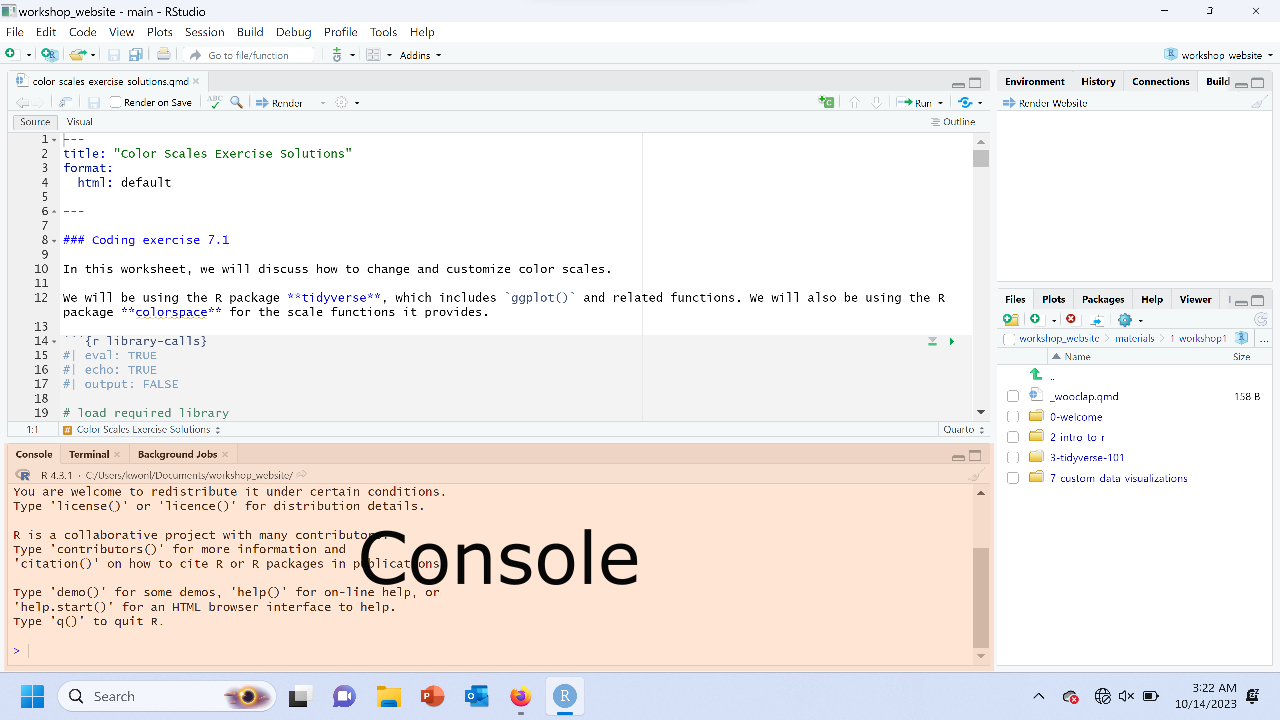
The console
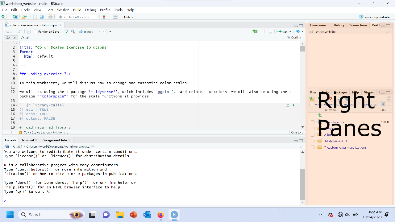
The right panes
Let’s take a poll
Go to the event on wooclap

M2. Match the areas with the right functionality
Let’s start programming
What is programming?
Programming is giving the computer instructions using text. The tricky part is learning how to speak to a computer.
```{r}
"a" == "A"
```
```{r error=TRUE}
max(c(1,2,3,4))
```
```{r error=TRUE}
# how old will I be in 10 years?
my_age + 10
```- Computers are incredibly literal
- Computers care about punctuation
[1] 4- Computers only know what you tell them
Error in eval(expr, envir, enclos): object 'my_age' not foundMost bugs happen because of one of these things.
What is programming?
So why bother at all? Because if you can tell a computer how to do it once, it is reproducible!
If the data changes or you find a mistake, just rerun!
You can run the same code on new data
You can share your code with others so they can start where you left off
Let’s use R for math
08:00
In the console, try typing some commands:
# arithmetic
3 + 5 + 10
10 * (5 + 1)
3**2 # what does the ** operator do in R?
# check inequalities and equalities
4 >= 1 # what does this mean?
5 + 4 == 9
# make some errors
"3" + 5 # why is this an error?
my_age + 5  # why is this an error?

# write a math expression to calculate what percentage
# of your life has been in post-secondary school/training
# (university, training programs, masters, PhD)
Say hello to the text-editor
When you write code in the console, it is gone.
It is better to work inside quarto notebooks in order to be able to save and share your code and results.
What can you do with Quarto?
Articles
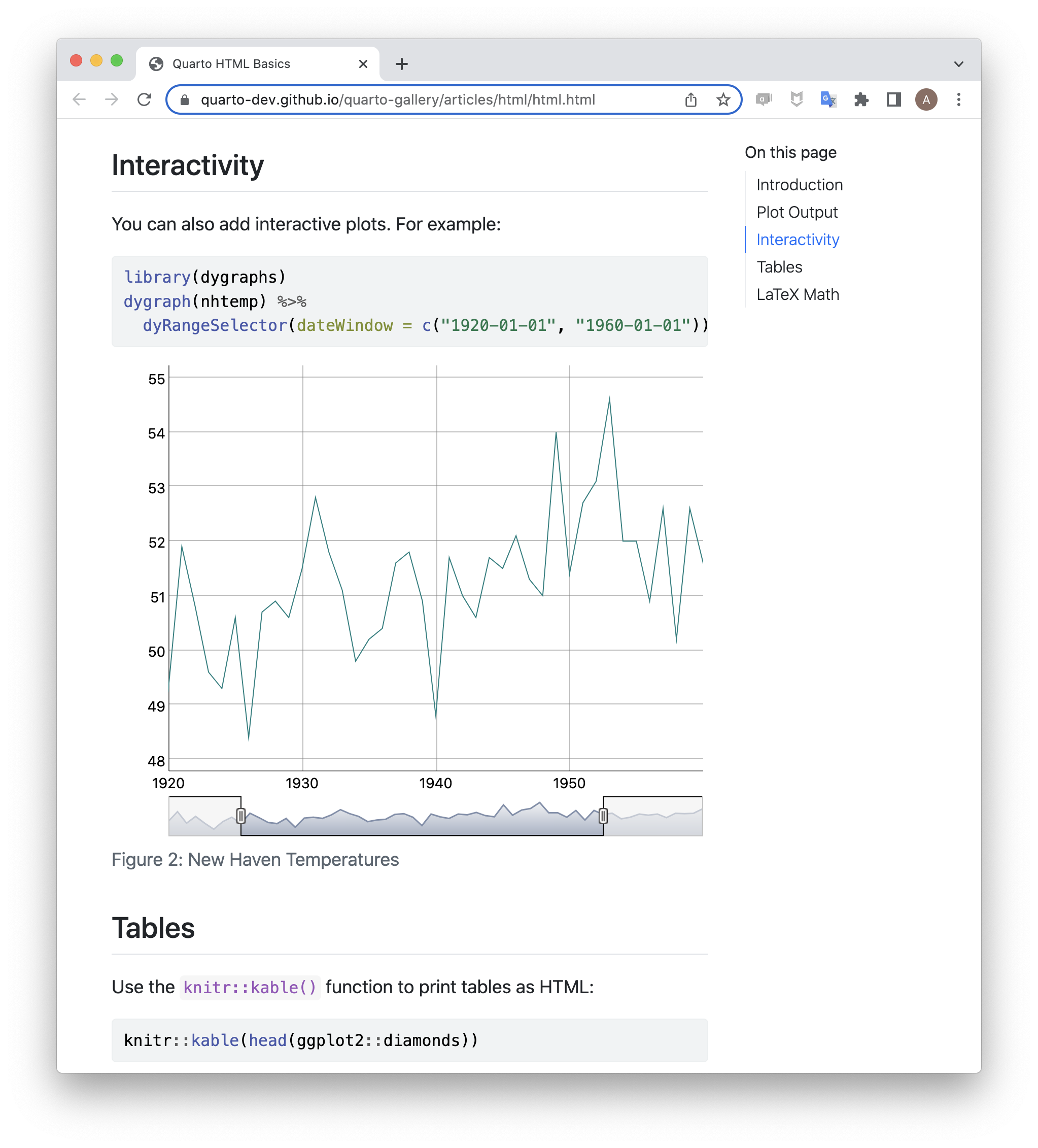
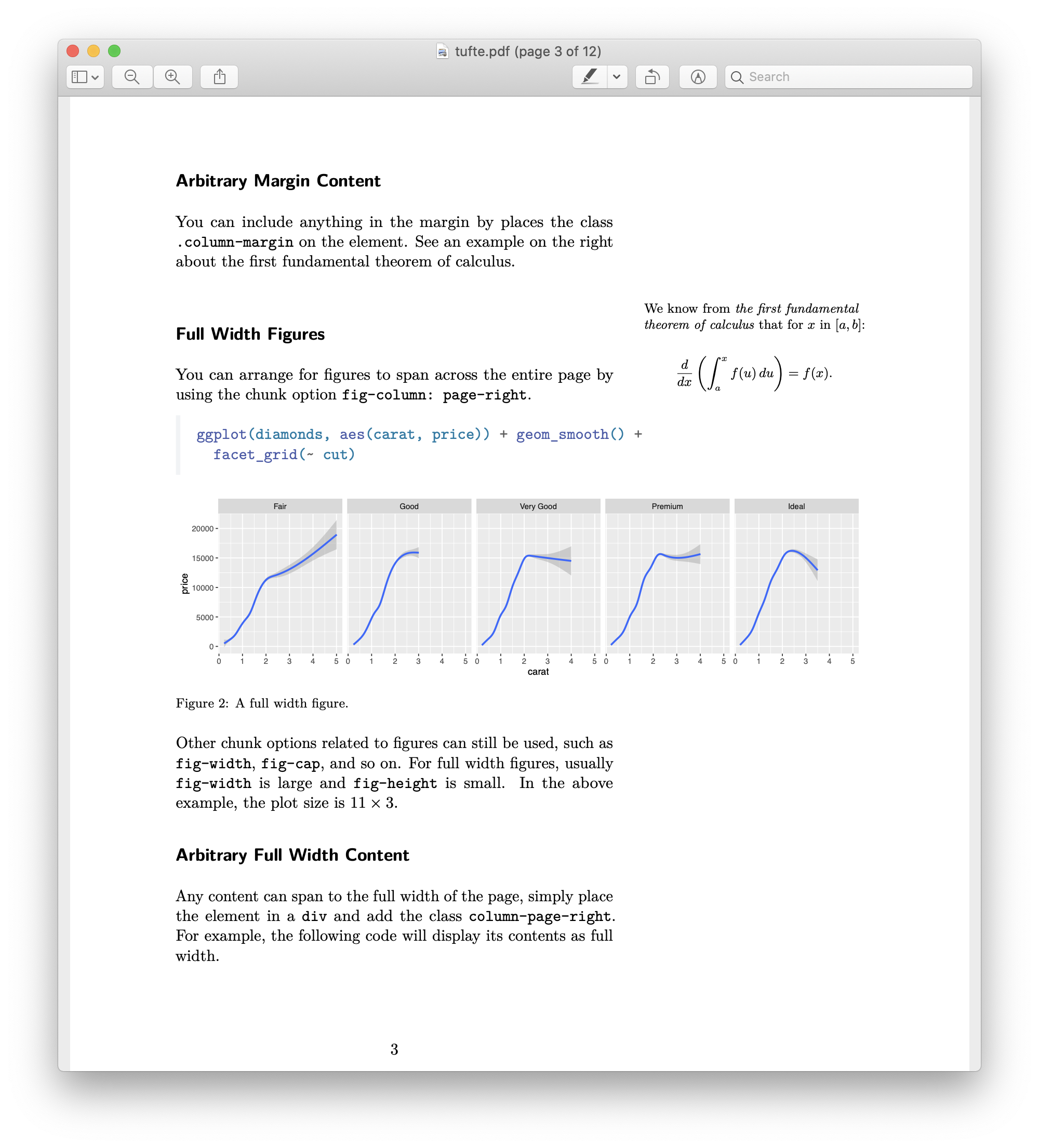
Presentations

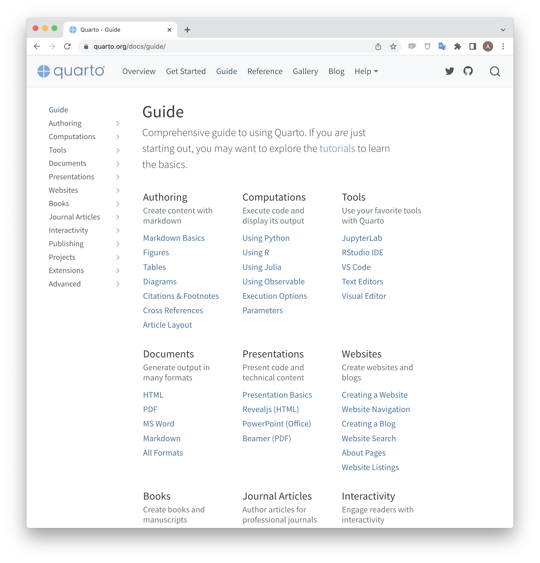
Websites

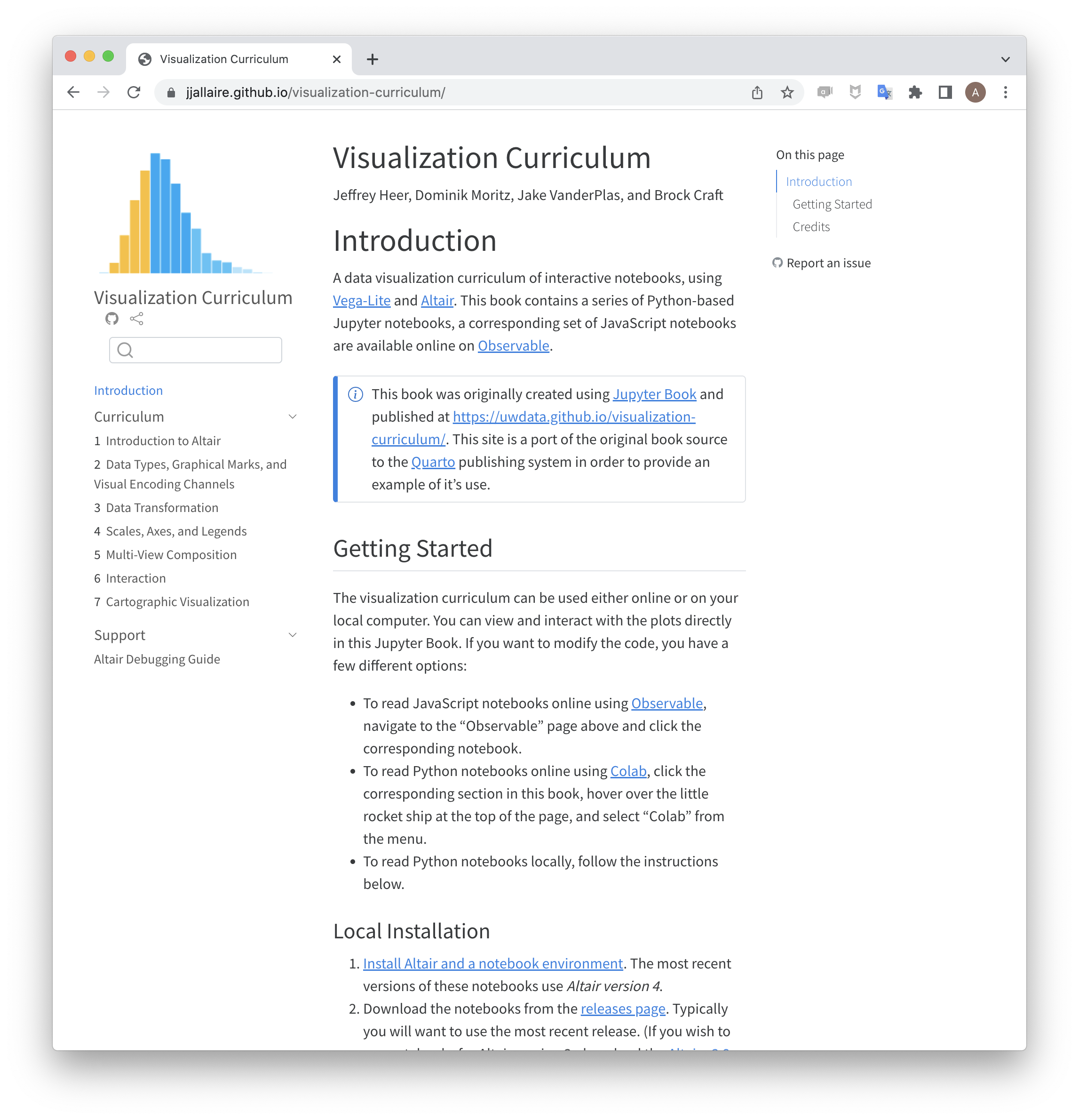
Books

Quarto Render
Quarto is integrated into RStudio
Click ![]() in Editor pane of RStudio.
in Editor pane of RStudio.
Render input file to various document formats.
Input
*.qmd*.ipynb*.md*.Rmd
Format
htmlpdfrevealjs(like these slides!)docxppt- and many more!
Anatomy of a Document
- Code Cells
- Text
- Metadata
Code Chunks
Quarto’s Code Chunk
This is a Quarto Code Chunk.
Let’s explore the survey data
Quarto’s Code Chunk
This is a Quarto Code Chunk.
Make a new code chunk in three ways:
- Type it out
- got to Code -> Insert Chunk on the top menu
- click in your document and hit the key combination
Alt+Ctrl+i
Write a math expression in a chunk and press the green arrow at the top-right of the chunk.
Execution Options
Control how the code is executed with options.
Options are denoted with the “hash-pipe” #|
| Option | Description |
|---|---|
eval |
Evaluate the code chunk (if false, just echos the code into the output). |
echo |
Include the source code in output |
output |
Include the results of executing the code in the output (true, false, or asis to indicate that the output is raw markdown and should not have any of Quarto’s standard enclosing markdown). |
warning |
Include warnings in the output. |
error |
Include errors in the output. |
include |
Catch all for preventing any output (code or results) from being included (e.g. include: false suppresses all output from the code block). |
Example: Figures from Code
Example: Figures from Code
Text
The Basics of Markdown
Markdown is designed to be easy to write and easy to read:
A Markdown-formatted document should be publishable as-is, as plain text, without looking like it’s been marked up with tags or formatting instructions.
-John Gruber
- Quarto uses extended version of Pandoc markdown.
- Pandoc classifies markdown in terms of Inline and Block elements.
Inline Elements: Text Formatting
Markdown
Output
Markdown allows you to format text with emphasis and strong emphasis. You can also add superscripts2, subscripts2, and display code verbatim. Little known fact: you can also strikethrough text and present it in small caps.
1
Inline Elements: Links and Images
Markdown
You can embed [links with names](https://quarto.org/), direct urls
like <https://quarto.org/>, and links to
[other places](#inline-elements-text-formatting) in the document.
The syntax is similar for embedding an inline image:
.
Output
You can embed links with names, direct urls like https://quarto.org/, and links to other places in the document. The syntax is similar for embedding an inline image: ![]() .
.
Markdown can do so much more
To learn about footnotes, Math, tables, and diagrams, check out the quarto documentation on markdown
Metadata: YAML
“Yet Another Markup Language” or “YAML Ain’t Markup Language” is used to provide document level metadata …
[… in key-value pairs,]
[… that can nest,]
[… are fussy about indentation,]
[… and are kept between ---.]
There are many options for front matter and configuring rendering.
Quarto + RStudio =
analysis code, documentation, and interpretation combined.
Ok, but how do you write code?
Assignment
You can use <- or = to assign values to variables
We will use <- for all examples going forward, but do whichever melts your brain less
Naming variables
A lot of R people use . inside variable names, but in most languages besides R this would be an error. It’s good practice these days to use the _ underscore if you want separation in your variable names.
Functions
Functions are named bits of code that take parameters as input and return some output
str_c is a function that puts concatenates strings.
Functions
Functions are named bits of code that take parameters as input and return some output
[1] "hello world"str_c is a function that puts concatenates strings.
functions can have named parameters as well as positional parameters.
Functions
Functions are named bits of code that take parameters as input and return some output
[1] "hello world"str_c is a function that puts concatenates strings.
functions can have named parameters as well as positional parameters.
named parameters always take an = sign for assignment.
Getting help with functions
Type ?str_c in the console to get a help page. check out this guide on how to read the R help pages.
also try googling str_c R tidyverse to get help.
chatGPT and phind.com are really good at answering specific questions about R functions - not always correct but most of the time.
“Everything is a vector”
This sounds like nonsense - let’s unpack:
- A Vector is a collection of values surrounded by
c()and separated with,
“Everything is a vector”
This sounds like nonsense - let’s unpack:
A vector is a collection of values surrounded by
c()and separated with,Vectors in R do smart things with most functions and operations.
“Everything is a vector”
This sounds like nonsense - let’s unpack:
A vector is a collection of values surrounded by
c()and separated with,Vectors in R do smart things with most functions and operations.
Vectors have only one type of value.
Value types in R
The type of the value can be
tibbles (aka data frames)
tibbles are the big reason R is great for working with tabular data.
A data frame is a rectangular collection of variables (in the columns) and observations (in the rows).
# A tibble: 132 × 6
   pid    time_point arm     nugent_score crp_blood    ph
   <chr>  <chr>      <chr>          <dbl>     <dbl> <dbl>
 1 pid_01 baseline   placebo            8      0.44   5.7
 2 pid_01 week_1     placebo            7      1.66   5.2
 3 pid_01 week_7     placebo            7      1.44   5.4
 4 pid_02 baseline   placebo            7      1.55   5.2
 5 pid_02 week_1     placebo            7      0.75   4.8
 6 pid_02 week_7     placebo            4      1.17   4.2
 7 pid_03 baseline   placebo            6      1.78   4.8
 8 pid_03 week_1     placebo           10      0.57   5.3
 9 pid_03 week_7     placebo            7      1.79   5.2
10 pid_04 baseline   placebo            5      1.76   4.8
# ℹ 122 more rows
Exercise
That’s enough slides for now time to try for yourself! Go to the module and go to the first exercise.
30:00
Elementary data manipulations
Pick rows:
filter()Pick columns:
select()Sort rows:
arrange()Count things:
count()Make new columns:
mutate()
How to read in data?
Data is often in tables, and the easiest way to store tabular data is in csv or tsv format.
csv - comma separated values
tsv - tab separated values
to read in data stored this way use read_csv(filename) or read_tsv(filename)
But first: the pipe operator %>%
But first: the pipe operator %>%
%>% is pronounced “and then”
The pipe %>% feeds data into functions
# A tibble: 6 × 6
  pid    time_point arm     nugent_score crp_blood    ph
  <chr>  <chr>      <chr>          <dbl>     <dbl> <dbl>
1 pid_01 baseline   placebo            8      0.44   5.7
2 pid_01 week_1     placebo            7      1.66   5.2
3 pid_01 week_7     placebo            7      1.44   5.4
4 pid_02 baseline   placebo            7      1.55   5.2
5 pid_02 week_1     placebo            7      0.75   4.8
6 pid_02 week_7     placebo            4      1.17   4.2
The pipe %>% feeds data into functions
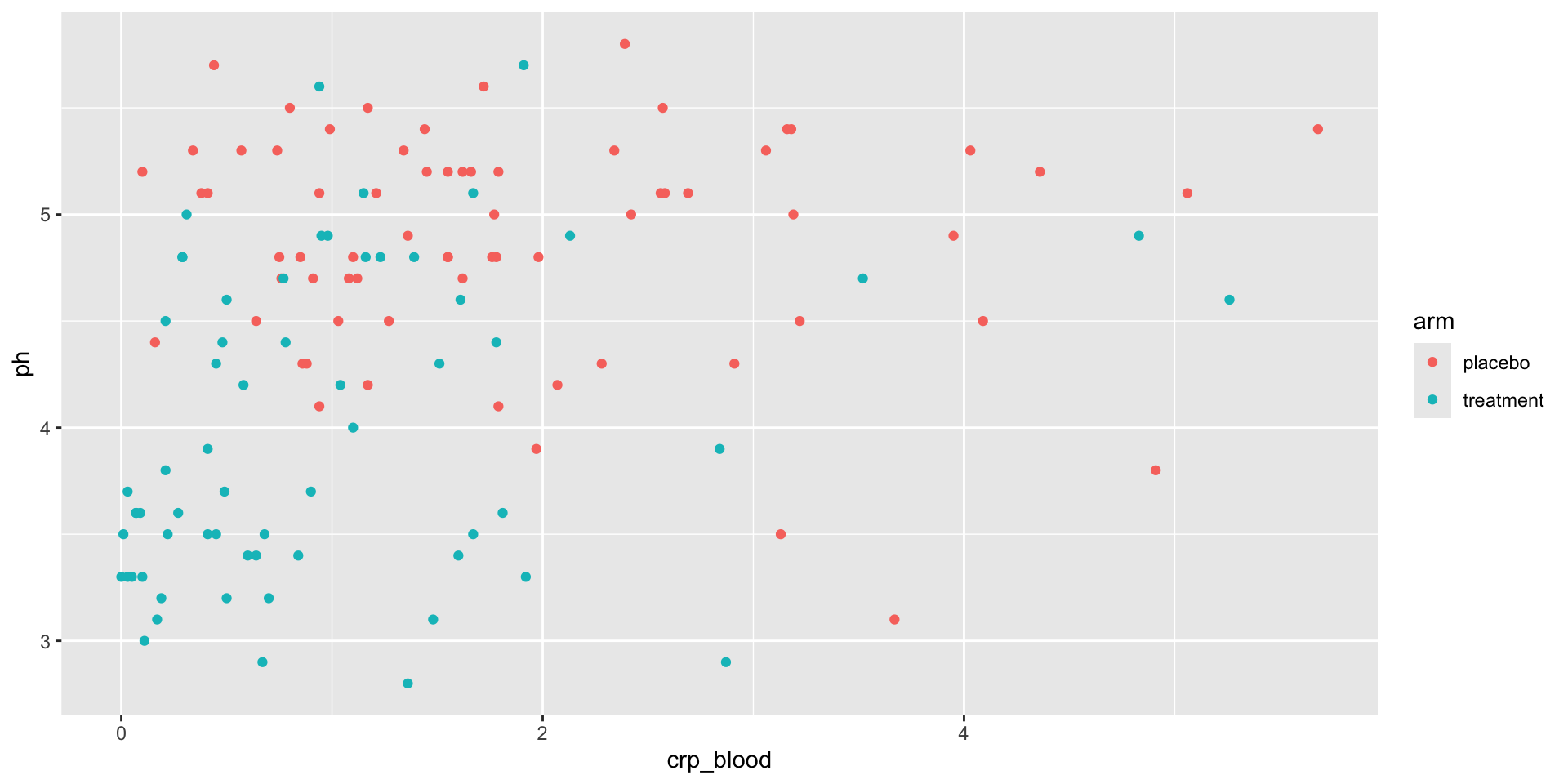
The pipe %>% feeds data into functions

Since R 4.1: Native pipe |>

Which to use? Native pipe or old-school pipe?
|>is the future. If you can, use it.%>%works on older installations. It’s the safe choice for now.
We use %>% here because many people still run older R versions. Also, we’re old school.
Picking rows or columns, and sorting
Pick rows from a table: filter()
Filter only placebo
# A tibble: 69 × 6
   pid    time_point arm     nugent_score crp_blood    ph
   <chr>  <chr>      <chr>          <dbl>     <dbl> <dbl>
 1 pid_01 baseline   placebo            8      0.44   5.7
 2 pid_01 week_1     placebo            7      1.66   5.2
 3 pid_01 week_7     placebo            7      1.44   5.4
 4 pid_02 baseline   placebo            7      1.55   5.2
 5 pid_02 week_1     placebo            7      0.75   4.8
 6 pid_02 week_7     placebo            4      1.17   4.2
 7 pid_03 baseline   placebo            6      1.78   4.8
 8 pid_03 week_1     placebo           10      0.57   5.3
 9 pid_03 week_7     placebo            7      1.79   5.2
10 pid_04 baseline   placebo            5      1.76   4.8
# ℹ 59 more rows
Filter out samples with ph < 4
# A tibble: 39 × 6
   pid    time_point arm       nugent_score crp_blood    ph
   <chr>  <chr>      <chr>            <dbl>     <dbl> <dbl>
 1 pid_05 week_1     treatment            3      0.19   3.2
 2 pid_05 week_7     treatment            2      0.45   3.5
 3 pid_09 week_1     treatment            3      0.27   3.6
 4 pid_10 week_1     treatment            0      0.01   3.5
 5 pid_10 week_7     treatment            1      2.87   2.9
 6 pid_11 week_1     treatment            1      0.1    3.3
 7 pid_15 week_1     treatment            3      0.84   3.4
 8 pid_15 week_7     treatment            3      0.68   3.5
 9 pid_16 week_1     treatment            0      0.03   3.7
10 pid_16 week_7     treatment            2      0.5    3.2
# ℹ 29 more rows
Pick columns from a table: select()
Pick columns pid, ph, and nugent
Rename columns and subset with select
# A tibble: 132 × 3
   participant_id    ph nugent_score
   <chr>          <dbl>        <dbl>
 1 pid_01           5.7            8
 2 pid_01           5.2            7
 3 pid_01           5.4            7
 4 pid_02           5.2            7
 5 pid_02           4.8            7
 6 pid_02           4.2            4
 7 pid_03           4.8            6
 8 pid_03           5.3           10
 9 pid_03           5.2            7
10 pid_04           4.8            5
# ℹ 122 more rows
Sort the rows in a table: arrange()
Sort samples by ph ascending
# A tibble: 132 × 6
   pid    time_point arm       nugent_score crp_blood    ph
   <chr>  <chr>      <chr>            <dbl>     <dbl> <dbl>
 1 pid_31 week_7     treatment            2      1.36   2.8
 2 pid_10 week_7     treatment            1      2.87   2.9
 3 pid_28 baseline   treatment            3      0.67   2.9
 4 pid_26 week_1     treatment            0      0.11   3
 5 pid_23 week_7     placebo              3      3.67   3.1
 6 pid_40 baseline   treatment            3      1.48   3.1
 7 pid_40 week_1     treatment            2      0.17   3.1
 8 pid_05 week_1     treatment            3      0.19   3.2
 9 pid_16 week_7     treatment            2      0.5    3.2
10 pid_37 week_7     treatment            2      0.7    3.2
# ℹ 122 more rows
Sort samples by ph, descending
# A tibble: 132 × 6
   pid    time_point arm       nugent_score crp_blood    ph
   <chr>  <chr>      <chr>            <dbl>     <dbl> <dbl>
 1 pid_29 baseline   placebo              7      2.39   5.8
 2 pid_01 baseline   placebo              8      0.44   5.7
 3 pid_16 baseline   treatment            6      1.91   5.7
 4 pid_06 week_1     placebo              8      1.72   5.6
 5 pid_26 baseline   treatment            7      0.94   5.6
 6 pid_13 week_1     placebo              7      2.57   5.5
 7 pid_23 week_1     placebo              8      0.8    5.5
 8 pid_27 baseline   placebo              7      1.17   5.5
 9 pid_01 week_7     placebo              7      1.44   5.4
10 pid_04 week_7     placebo              7      5.68   5.4
# ℹ 122 more rows
Counting things
To demonstrate counting, let’s switch to table_01
# A tibble: 44 × 6
   pid    arm       smoker       age education                     sex
   <chr>  <chr>     <chr>      <dbl> <chr>                         <lgl>
 1 pid_01 placebo   non-smoker    26 grade 10-12, matriculated     FALSE
 2 pid_02 placebo   smoker        33 grade 10-12, matriculated     FALSE
 3 pid_03 placebo   smoker        30 post-secondary                FALSE
 4 pid_04 placebo   non-smoker    34 grade 10-12, not matriculated FALSE
 5 pid_05 treatment non-smoker    29 grade 10-12, matriculated     FALSE
 6 pid_06 placebo   smoker        34 post-secondary                FALSE
 7 pid_07 placebo   non-smoker    31 grade 10-12, not matriculated FALSE
 8 pid_08 placebo   smoker        30 grade 10-12, not matriculated FALSE
 9 pid_09 treatment non-smoker    35 grade 10-12, not matriculated FALSE
10 pid_10 treatment non-smoker    32 less than grade 9             FALSE
# ℹ 34 more rows
Counting things
Counting things
Let’s take a poll
Go to the event on wooclap

M2. Does filter get rid of rows that match TRUE, or keep rows that match TRUE?
Use the pipe to build analysis pipelines
# A tibble: 23 × 6
   pid    arm     smoker       age education                     sex
   <chr>  <chr>   <chr>      <dbl> <chr>                         <lgl>
 1 pid_01 placebo non-smoker    26 grade 10-12, matriculated     FALSE
 2 pid_02 placebo smoker        33 grade 10-12, matriculated     FALSE
 3 pid_03 placebo smoker        30 post-secondary                FALSE
 4 pid_04 placebo non-smoker    34 grade 10-12, not matriculated FALSE
 5 pid_06 placebo smoker        34 post-secondary                FALSE
 6 pid_07 placebo non-smoker    31 grade 10-12, not matriculated FALSE
 7 pid_08 placebo smoker        30 grade 10-12, not matriculated FALSE
 8 pid_12 placebo non-smoker    31 grade 10-12, matriculated     FALSE
 9 pid_13 placebo non-smoker    32 post-secondary                FALSE
10 pid_14 placebo smoker        32 grade 10-12, matriculated     FALSE
# ℹ 13 more rows
Use the pipe to build analysis pipelines
# A tibble: 12 × 3
   pid    arm       smoker
   <chr>  <chr>     <chr>
 1 pid_01 placebo   non-smoker
 2 pid_05 treatment non-smoker
 3 pid_15 treatment non-smoker
 4 pid_17 treatment non-smoker
 5 pid_21 treatment non-smoker
 6 pid_27 placebo   smoker
 7 pid_30 placebo   non-smoker
 8 pid_31 treatment non-smoker
 9 pid_35 placebo   non-smoker
10 pid_36 placebo   non-smoker
11 pid_41 treatment smoker
12 pid_44 treatment non-smoker
Use the pipe to build analysis pipelines
Adding new columns to a table
Make a new table column: mutate()
Example: C-reactive protein
The crp_blood column is in units of mg/L. What if you needed it in ug/ul? What’s the calculation?
# A tibble: 132 × 3
   pid    time_point crp_blood
   <chr>  <chr>          <dbl>
 1 pid_01 baseline        0.44
 2 pid_01 week_1          1.66
 3 pid_01 week_7          1.44
 4 pid_02 baseline        1.55
 5 pid_02 week_1          0.75
 6 pid_02 week_7          1.17
 7 pid_03 baseline        1.78
 8 pid_03 week_1          0.57
 9 pid_03 week_7          1.79
10 pid_04 baseline        1.76
# ℹ 122 more rows
Example: C-reactive protein
The crp_blood column is in units of mg/L. What if you needed it in ug/ul? What’s the calculation?
To get ug/L you would multiply by 1000. To get ug/ul you need to then divide by 1000000
```{r}
table_02 %>%
  select(pid, time_point, crp_blood) %>%
  mutate(crp_blood_ugul = crp_blood / 1000)
```
# A tibble: 132 × 4
pid time_point crp_blood crp_blood_ugul
<chr> <chr> <dbl> <dbl>
1 pid_01 baseline 0.44 0.00044
2 pid_01 week_1 1.66 0.00166
3 pid_01 week_7 1.44 0.00144
4 pid_02 baseline 1.55 0.00155
5 pid_02 week_1 0.75 0.00075
6 pid_02 week_7 1.17 0.00117
7 pid_03 baseline 1.78 0.00178
8 pid_03 week_1 0.57 0.00057
9 pid_03 week_7 1.79 0.00179
10 pid_04 baseline 1.76 0.00176
# ℹ 122 more rowsMake multiple columns at once
```{r}
table_02 %>%
  select(pid, time_point, crp_blood) %>%
  mutate(crp_blood_ugul = crp_blood / 1000,
         crp_blood_ugl = crp_blood * 1000)
```
# A tibble: 132 × 5
pid time_point crp_blood crp_blood_ugul crp_blood_ugl
<chr> <chr> <dbl> <dbl> <dbl>
1 pid_01 baseline 0.44 0.00044 440
2 pid_01 week_1 1.66 0.00166 1660
3 pid_01 week_7 1.44 0.00144 1440
4 pid_02 baseline 1.55 0.00155 1550
5 pid_02 week_1 0.75 0.00075 750
6 pid_02 week_7 1.17 0.00117 1170
7 pid_03 baseline 1.78 0.00178 1780
8 pid_03 week_1 0.57 0.00057 570
9 pid_03 week_7 1.79 0.00179 1790
10 pid_04 baseline 1.76 0.00176 1760
# ℹ 122 more rowsExercise
That’s enough slides for now time to try for yourself! Go to the module and go to the second exercise.
30:00
