| Characteristic | Overall N = 271 |
birth_control N = 151 |
no_birth_control N = 121 |
p-value2 |
|---|---|---|---|---|
| Age (years) | 31.00 (30.00, 33.00) | 31.00 (29.00, 33.00) | 31.50 (30.00, 33.00) | 0.5 |
| PCOS status | 0.2 | |||
| no disease | 13 (48%) | 9 (60%) | 4 (33%) | |
| pcos | 14 (52%) | 6 (40%) | 8 (67%) | |
| Period product | 0.8 | |||
| menstrual_cup | 4 (15%) | 2 (13%) | 2 (17%) | |
| pad | 4 (15%) | 3 (20%) | 1 (8.3%) | |
| tampon | 19 (70%) | 10 (67%) | 9 (75%) | |
| 1 Median (Q1, Q3); n (%) | ||||
| 2 Wilcoxon rank sum test; Pearson’s Chi-squared test; Fisher’s exact test | ||||
The vaginal immune environment across the menstrual cycle
An example group-project presentation · Group B
Part 1 · The dataset
The study
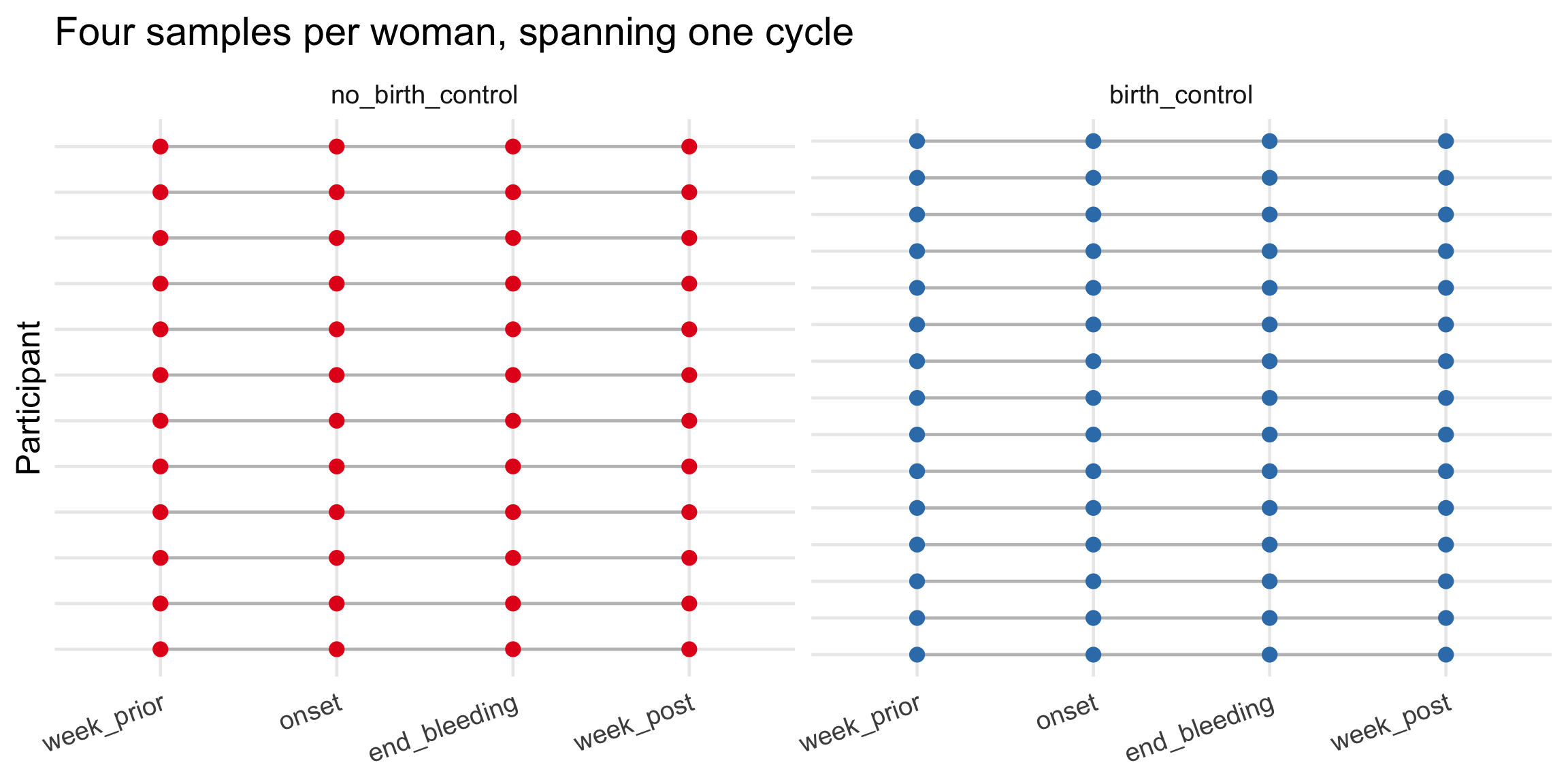
An observational study of 27 women, 15 using hormonal birth control and 12 not. Each woman was sampled at four points across one menstrual cycle:
the week before bleeding → onset → end of bleeding → the week after
From each sample we have:
- Luminex — 8 cytokines (inflammation markers)
- flow cytometry — counts of immune cell types (neutrophils, T cells, …)
- participant metadata — age, PCOS status, period product
Two questions: how does the vaginal immune environment shift across the cycle, and does birth control change it?
Who is in the study?
This is a small cohort, so categorical rows use Fisher’s exact test.
How the study is laid out
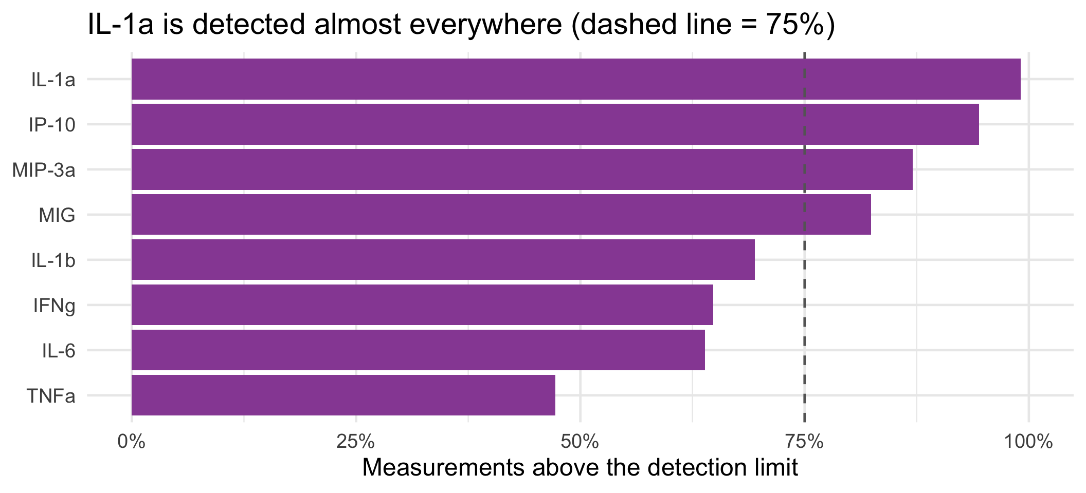
Which cytokines can we use?
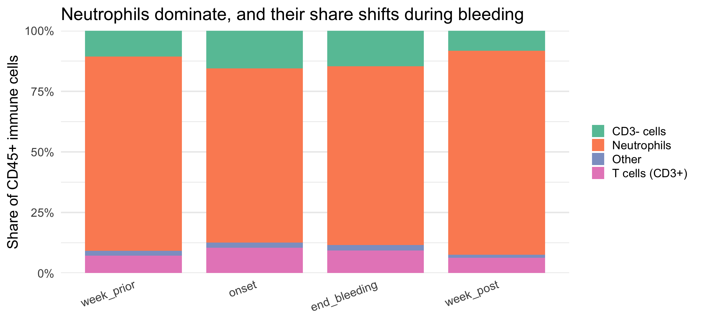
What the immune cells look like
Part 2 · Three short analyses
Three questions
- Does inflammation (IL-1a) rise during menstruation?
- Does the neutrophil share of immune cells change across the cycle?
- Does birth control shift the cytokine milieu?
Story 1 · Inflammation across the cycle
The question
Bleeding is a tissue-remodelling event, so we expect inflammation to track it.
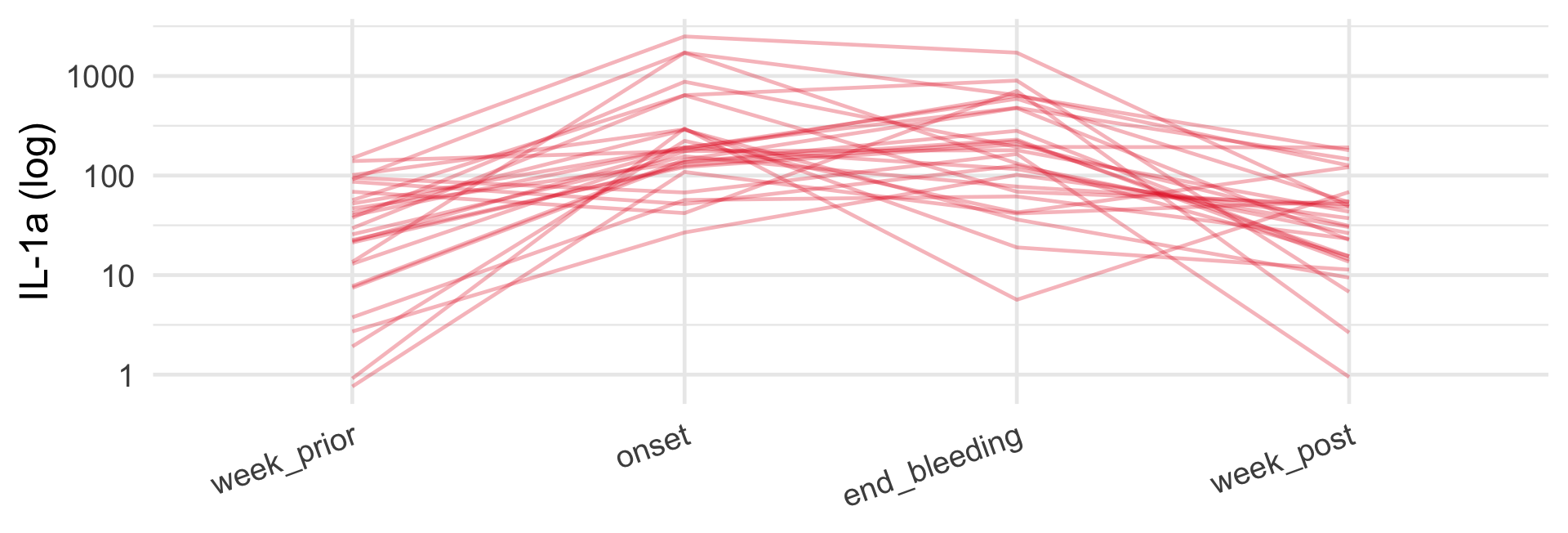
Does IL-1a rise during menstruation and settle afterwards? Each woman is measured four times, so we fit a model with a per-participant random effect and let the week-before-bleeding be the reference point.
The code
time_point is a factor ordered from the week before bleeding, so every coefficient reads as a change relative to that baseline week. (1 | pid) accounts for the four correlated samples per woman.
The table
| Term | Beta | 95% CI | p-value |
|---|---|---|---|
| (Intercept) | 3.1 | 2.6, 3.6 | <0.001 |
| time_point | |||
| week_prior | — | — | |
| onset | 2.3 | 1.6, 2.9 | <0.001 |
| end_bleeding | 2.0 | 1.4, 2.7 | <0.001 |
| week_post | 0.30 | -0.36, 0.95 | 0.4 |
| Abbreviation: CI = Confidence Interval | |||
What it means
On the log scale, relative to the week before bleeding:
- Onset: +2.3 — roughly a tenfold jump in IL-1a (p < 0.001).
- End of bleeding: +2.0 — still strongly elevated.
- Week after: +0.3 — back to baseline (p = 0.4).
Inflammation rises sharply with bleeding and resolves within a week. The cytokine milieu is a moving target that depends entirely on when in the cycle you sample — a key lesson for designing studies like this one.
Story 2 · Neutrophils across the cycle
The question
The Part 1 overview hinted that neutrophils’ share of immune cells changes during bleeding. Let’s test it properly.
The outcome is a proportion of counted cells, so the natural model is binomial — exactly the flow-cytometry recipe from the modeling lecture. Because the cell counts are huge, a plain binomial is wildly overconfident, so we add a per-sample random effect to capture the real sample-to-sample spread.
The code
flow <- flow |> mutate(other = cd45_positive - neutrophils)

fit <- glmer(
  cbind(neutrophils, other) ~ time_point + (1 | pid) + (1 | sample_id),
  family = binomial(), data = flow
)

# the figure: observed neutrophil share across the cycle
ggboxplot(flow, x = "time_point", y = "prop_neut",
          fill = "time_point", palette = "Set1") +
  stat_compare_means(method = "wilcox.test", ref.group = "week_prior",
                     label = "p.signif")
The figure
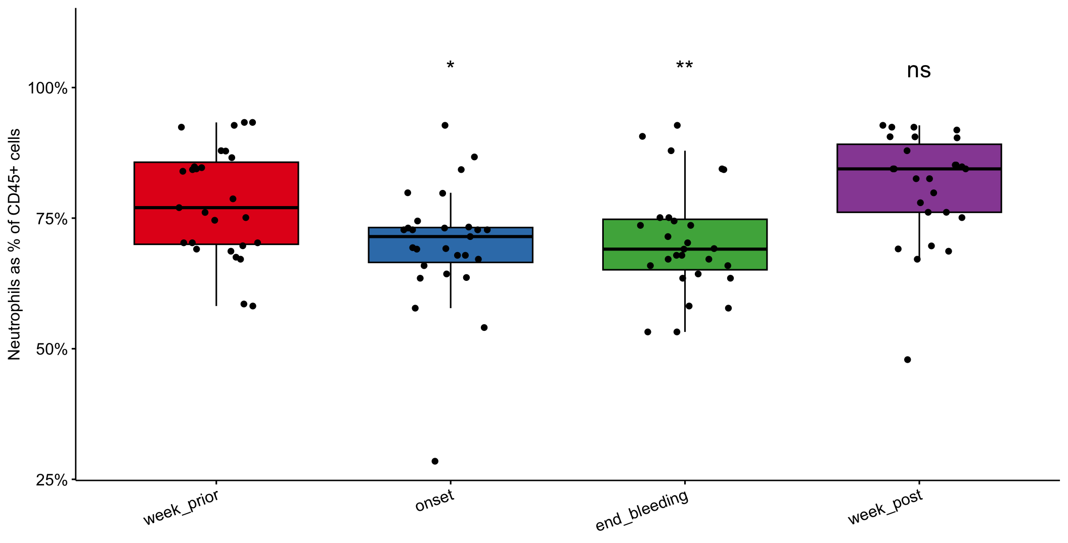
Stars compare each timepoint to the week before bleeding (ns = not significant).
What it means
| Term | log(OR) | 95% CI | p-value |
|---|---|---|---|
| time_point | |||
| week_prior | — | — | |
| onset | -0.49 | -0.83, -0.16 | 0.004 |
| end_bleeding | -0.44 | -0.77, -0.10 | 0.010 |
| week_post | 0.20 | -0.13, 0.53 | 0.2 |
| Abbreviations: CI = Confidence Interval, OR = Odds Ratio | |||
- The neutrophil share dips at onset and end of bleeding and is highest again the week after (model p ≈ 0.004 and 0.01).
- The per-sample random effect was essential: without it the model treats hundreds of thousands of cells as independent coin flips and reports impossibly tiny p-values.
- Participant-to-participant variation was near zero — the cycle stage, not the individual, drives the neutrophil share.
Story 3 · Does birth control matter?
The question
Hormonal contraception changes the cervicovaginal environment, so we might expect it to leave a cytokine signature.
Does any cytokine differ between the birth-control and no-birth-control arms? We screen the well-detected cytokines and correct for multiple testing.
The code
keep <- c("IL-1a", "IP-10", "MIP-3a", "MIG")   # detected in >75% of samples

panel <- cyt |> filter(limits == "not_censored", cytokine %in% keep)

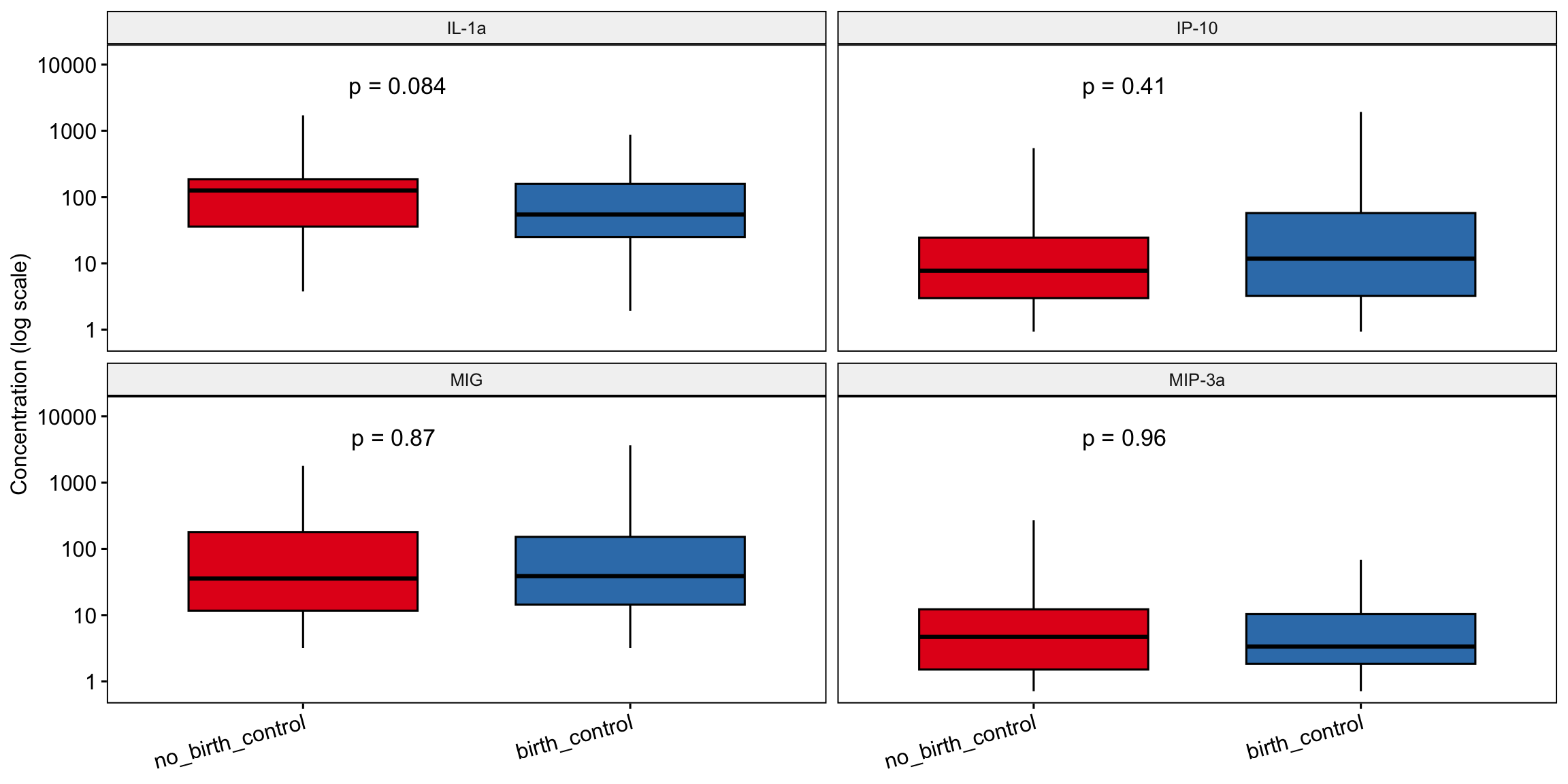
ggboxplot(panel, x = "arm", y = "conc", fill = "arm",
          palette = "Set1", facet.by = "cytokine") +
  scale_y_log10(expand = expansion(mult = c(0.05, 0.2))) +
  stat_compare_means(method = "wilcox.test", label = "p.format")
The figure
What it means
| Cytokine | n | p | p (BH) |
|---|---|---|---|
| IL-1a | 107 | 0.084 | 0.335 |
| IP-10 | 102 | 0.409 | 0.818 |
| MIG | 89 | 0.871 | 0.960 |
| MIP-3a | 94 | 0.960 | 0.960 |
No cytokine survives correction — not even before it. In this cohort, the menstrual cycle is a far stronger driver of the immune environment than birth control is. A null result, honestly reported, is still a finding.
Wrap-up
What we found
- Inflammation rises and falls with bleeding — IL-1a jumps ~10x at onset and resets within a week.
- Neutrophils’ share of immune cells dips during bleeding, then rebounds.
- Birth control left no detectable cytokine signature against that much larger cyclic signal.
The takeaway
Timing dominates. Any study of the vaginal immune environment has to account for cycle stage before it can ask about anything else.
Every table and figure here came from the workshop’s own toolkit — tidyverse, gtsummary, ggpubr, and lme4 — built with an LLM assistant, with the scientific judgement kept firmly in human hands.