Modeling and Uncertainty

Building models for biological data

Kris Sankaran and Marothi Peter Letsoalo

Practicalities

WiFi:

Network: Southernsunconference

Network Password: ahri2026

Previous password (only if ahri2026 doesn’t work): S0uthernsun1

Workshop materials are at:

https://elsherbini.github.io/data-science-for-biology/

Goals for this session

1. Distinguish between the “large” and “small” worlds of modeling.

2. Compare biostatistical models and explain when they apply.

3. Use R to estimate models and know how to explain the output.

4. Diagnose and address model failures.

Part 1: What is a Model?

Let’s start with a picture

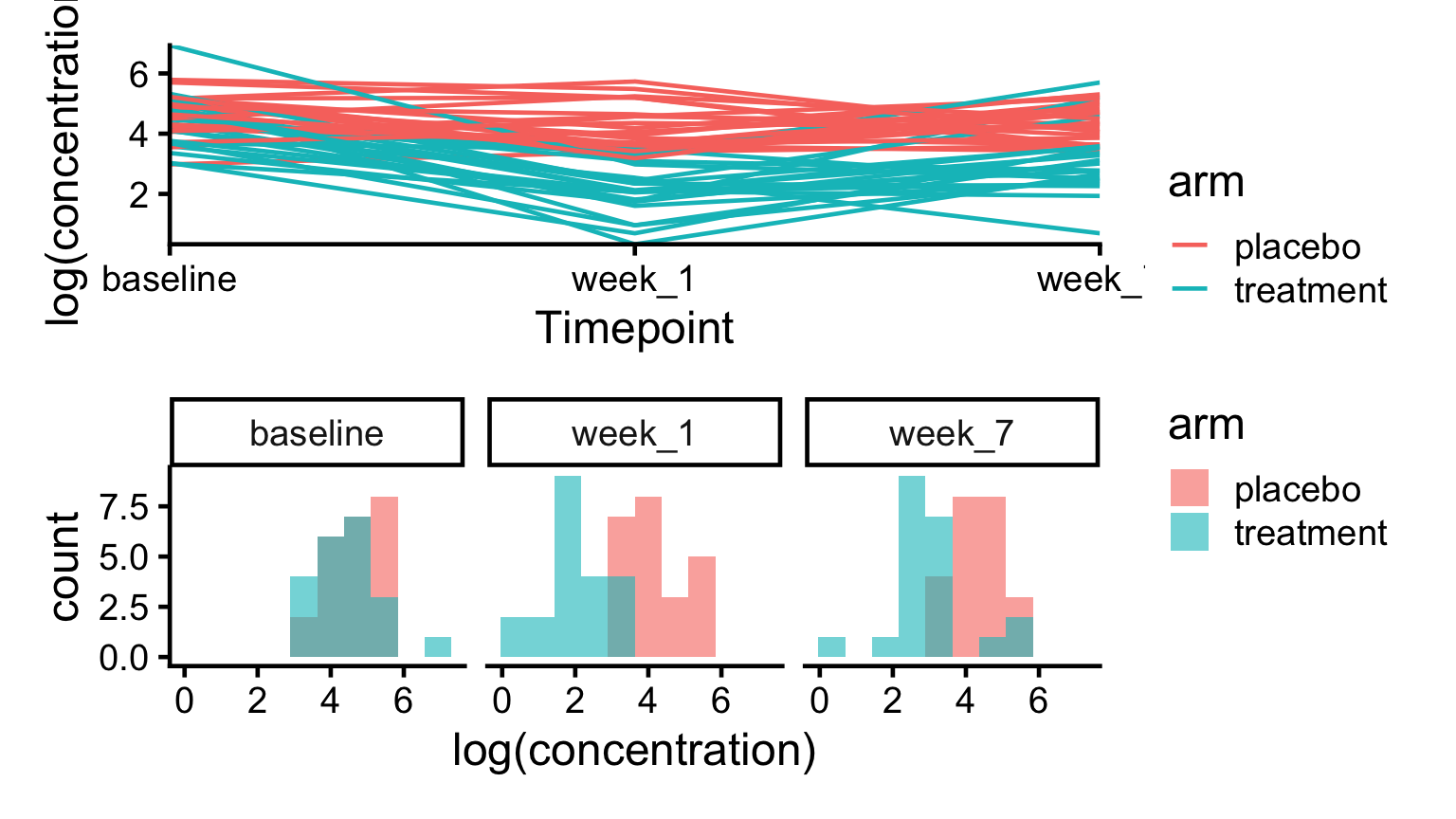
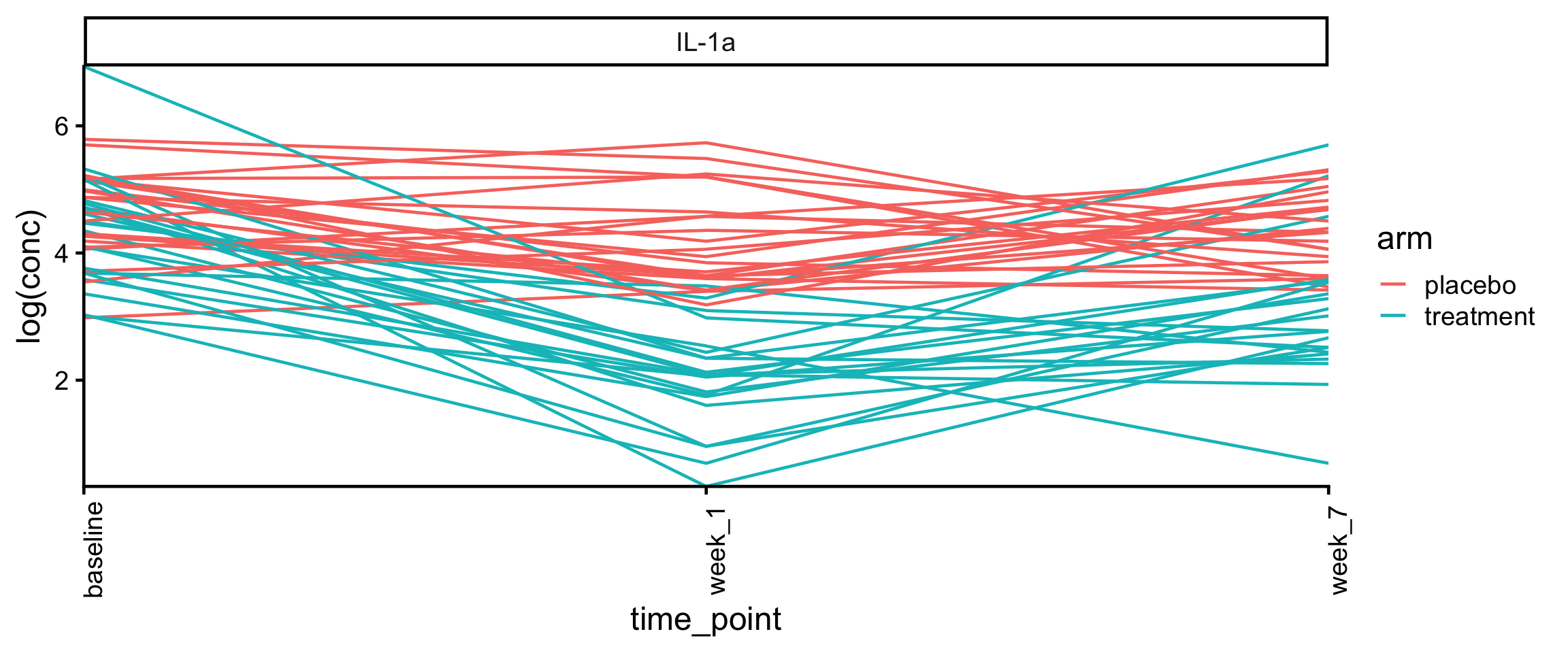
• The plots below show IL-1a concentration from our workshop luminex dataset.

• Notice the variation across people and a possible treatment effect at the post-treatment visit.

Discussion

Imagine running the study again, keeping the recruitment and experimental protocols as similar as possible. Make two lists:

• Aspects of the plots that you think will still be true in the new experiment.
• Aspects of the plots that you think will change.

A statistical model

A statistical model is a simplified description of how the data were generated, the “data story.”

• Model parameters let us answer scientific questions, like how a treatment affects outcomes.

• We observe just one realization of the data generating process – things could have turned out differently if we ran the study again.

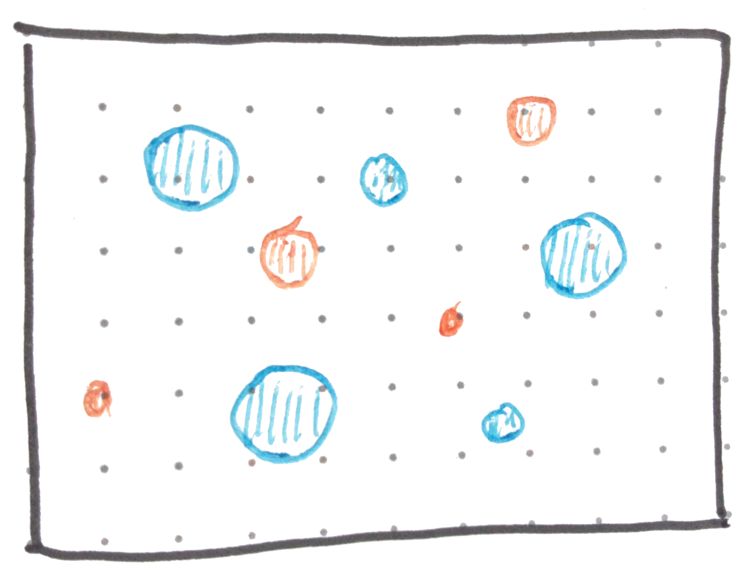
Large vs. small worlds

Large world

• Where the data were actually gathered
• Complex, influenced by factors we never observed
• Hard to carry out controlled interventions

Small world

• Inside the statistical model
• Logically consistent with precisely stated assumptions
• Allows hypothetical interventions and quantifies uncertainty

There will always be a gap between the two worlds. That gap is itself a source of uncertainty not captured by the model.

Large Worlds

A dataset is like a photograph of a biological system, but it develops slowly and is more error prone.

Large Worlds

A dataset is like a photograph of a biological system, but the snapshot takes longer to generate and is more error prone.

Large Worlds

A dataset is like a photograph of a biological system, but the snapshot takes longer to generate and is more error prone.

Small Worlds

• The small-world model summarizes what would stay true if the experiment were repeated.

• It encodes a data generating process that lets us simulate new data with the experiment’s key features, without memorizing every sample.

Modeling Checklist

1. Biological Question. What real-world questions do you want to answer?

2. Plot the Data. What does the outcome look like? Do you notice relationships with other variables?

3. Working Assumptions. Make a small-world story for how the data were generated. This is the initial statistical model.

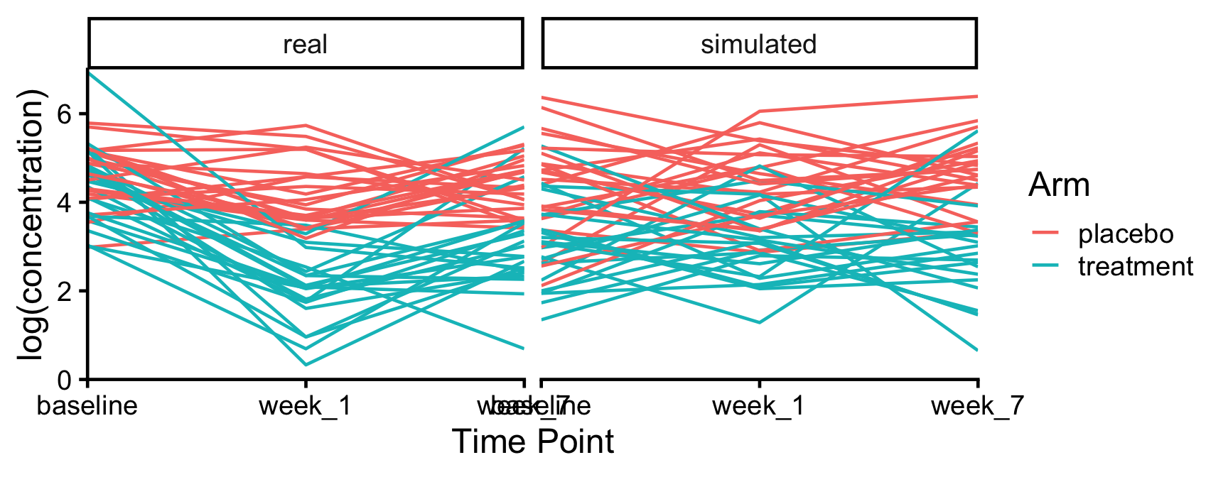
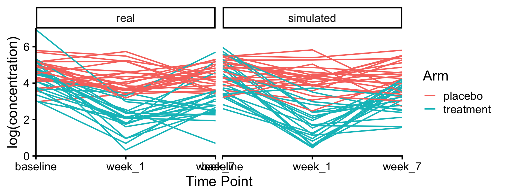
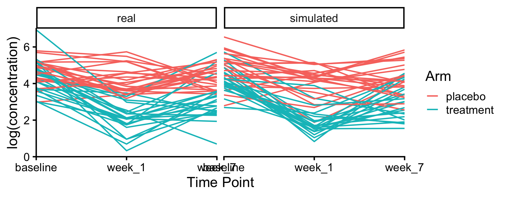
4. Model Checks. Use simulation and diagnostics to check whether the model captures patterns we see in the real data.

5. Revised Models. Revise until the model provides a good match. Use this to answer the original question.

Part 2: Basic Ingredients

Recipes

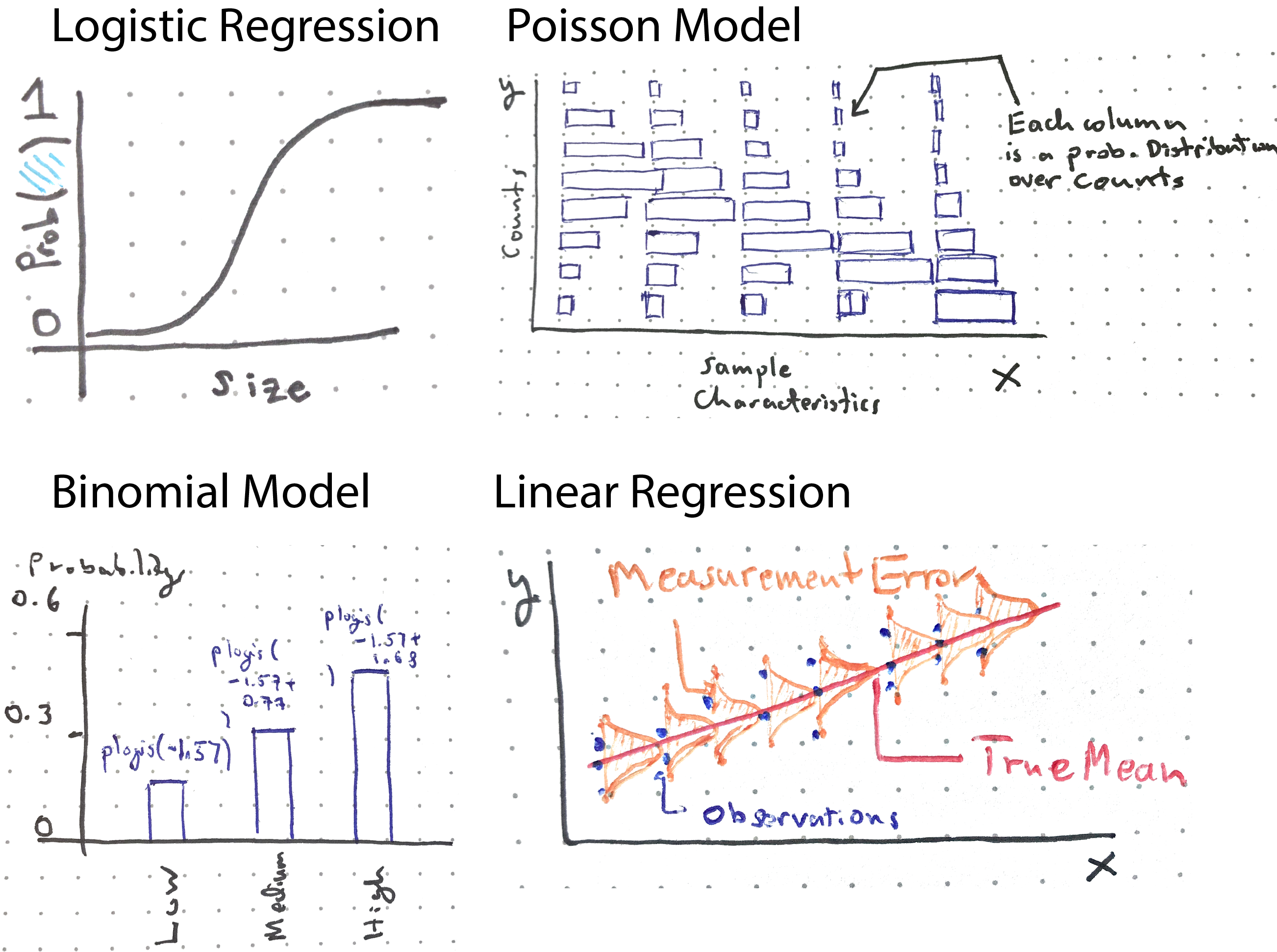
Each type of statistical model is designed for a different kind of data or biological question.

Like having a well-stocked pantry is needed to cook many recipes, knowing the basic statistical ingredients will allow you to adapt to whatever data or questions you encounter.

Today’s tour:

• Bernoulli — binary outcomes
• Poisson — count outcomes
• Linear regression — continuous outcomes
• Variations — multiple predictors, mixed effects, interactions

Bernoulli and Binomial Models

These models apply when outcomes fall into two groups.

• Heads vs. tails
• Infected vs. not infected
• Responder vs. non-responder
• CD3- cell vs. not CD3- cell

The Bernoulli is for individual outcomes, the Binomial applies to their totals

Bernoulli and Binomial Models

The raw data come from two classes, and we want their relative probabilities.

Bernoulli and Binomial Models

The raw data come from two classes, and we want their relative probabilities.

Model Covariates

The outcome probabilities can depend on sample-level covariates.

Model Covariates

The outcome probabilities can depend on sample-level covariates.

Infection data

• Each row corresponds to a person
• The outcome takes one of two values

Table 1

infections |>
    select(sample_id, social_contact, infected)

# A tibble: 100 × 3
   sample_id social_contact infected
   <chr>              <dbl>    <dbl>
 1 sample_1          0.748         1
 2 sample_2          0.379         0
 3 sample_3          0.483         0
 4 sample_4          0.813         0
 5 sample_5          0.670         0
 6 sample_6          0.400         0
 7 sample_7          0.0899        0
 8 sample_8          0.611         1
 9 sample_9          0.935         0
10 sample_10         0.849         1
# ℹ 90 more rows

Small World Model

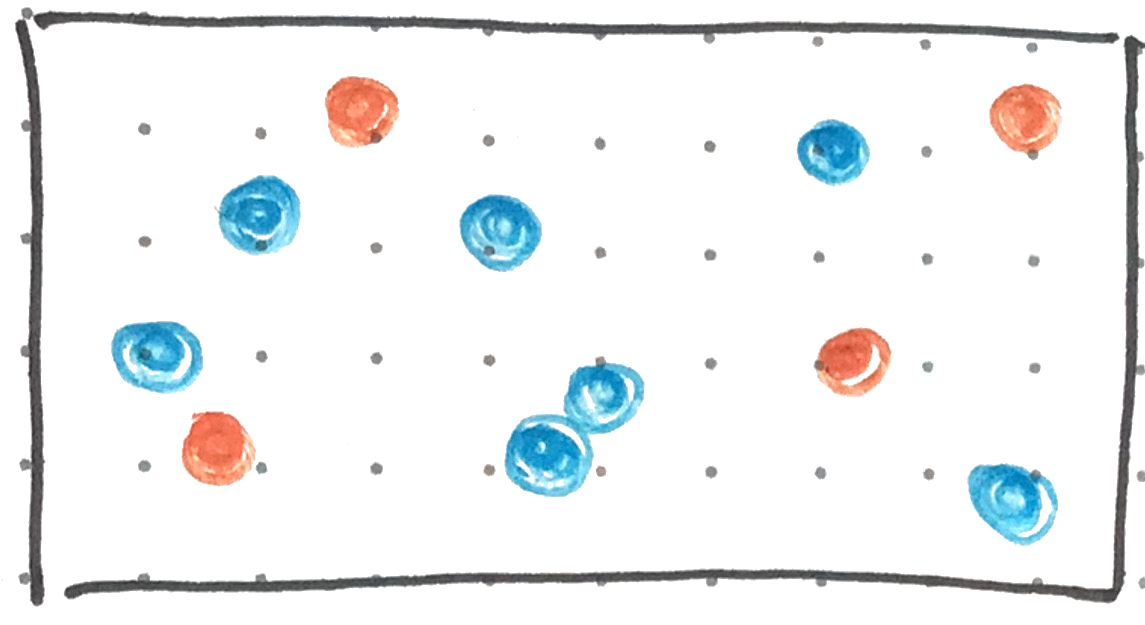
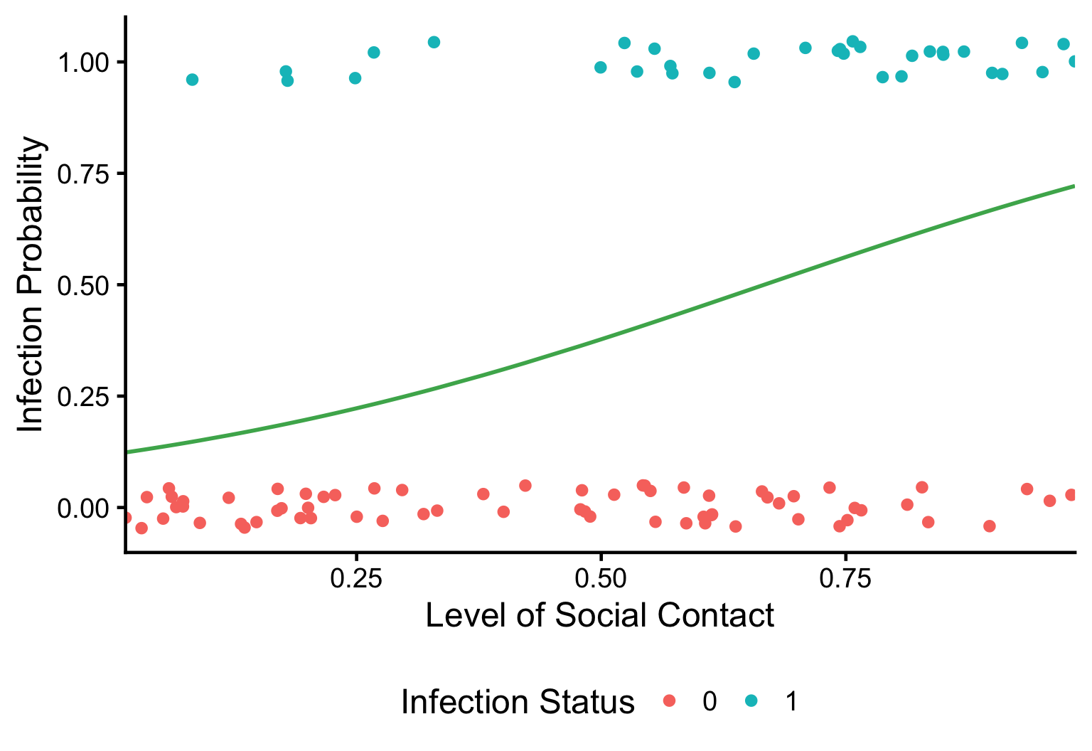
Data Story: More social contact → higher probability of infection.

• Response \(y\): Who does (1) or doesn’t (0) get infected during an outbreak?

• Covariates \(x\): Some people have larger social networks than others.

Fitting with glm

The glm function has three arguments:

• formula: written y ~ x, this relates outcome y to covariates x
• family: the type of model (depends on the data type of the outcome)
• data: a data.frame containing the columns named in formula

Bernoulli fit

fit <- glm(infected ~ social_contact, family = binomial(), data = infections)
summary(fit)

Call:
glm(formula = infected ~ social_contact, family = binomial(), 
    data = infections)

Coefficients:
               Estimate Std. Error z value Pr(>|z|)    
(Intercept)     -2.3702     0.5739  -4.130 3.63e-05 ***
social_contact   3.0933     0.8908   3.473 0.000515 ***
---
Signif. codes:  0 '***' 0.001 '**' 0.01 '*' 0.05 '.' 0.1 ' ' 1

(Dispersion parameter for binomial family taken to be 1)

    Null deviance: 128.21  on 99  degrees of freedom
Residual deviance: 113.69  on 98  degrees of freedom
AIC: 117.69

Number of Fisher Scoring iterations: 4

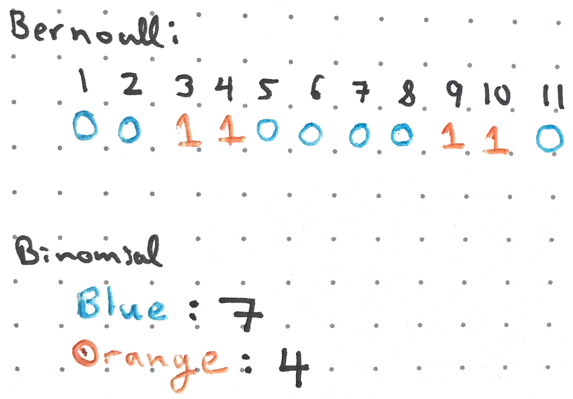
We wrote family = binomial(), but since infected is 0/1, the code knows to run a Bernoulli model.

Interpreting the fit

• The estimates are on the log-odds scale, which isn’t directly interpretable.

• plogis() converts them to the probability scale:

• This model is often called logistic regression, after the inverse logistic function (plogis).

Interpreting the fit

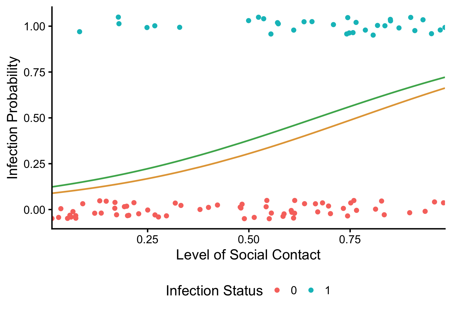
At social contact level x, the infection probability ≈ plogis(-2.37 + 3.09x)

• x = 0 \(\implies\) plogis(-2.37) ≈ 0.085
• x = 0.5 \(\implies\) plogis(-2.37 + 3.09 * 0.5) ≈ 0.24
• x = 1 \(\implies\) plogis(-2.37 + 3.09 * 1) ≈ 0.50

summary(fit)

Call:
glm(formula = infected ~ social_contact, family = binomial(), 
    data = infections)

Coefficients:
               Estimate Std. Error z value Pr(>|z|)    
(Intercept)     -2.3702     0.5739  -4.130 3.63e-05 ***
social_contact   3.0933     0.8908   3.473 0.000515 ***
---
Signif. codes:  0 '***' 0.001 '**' 0.01 '*' 0.05 '.' 0.1 ' ' 1

(Dispersion parameter for binomial family taken to be 1)

    Null deviance: 128.21  on 99  degrees of freedom
Residual deviance: 113.69  on 98  degrees of freedom
AIC: 117.69

Number of Fisher Scoring iterations: 4

Interpreting the fit

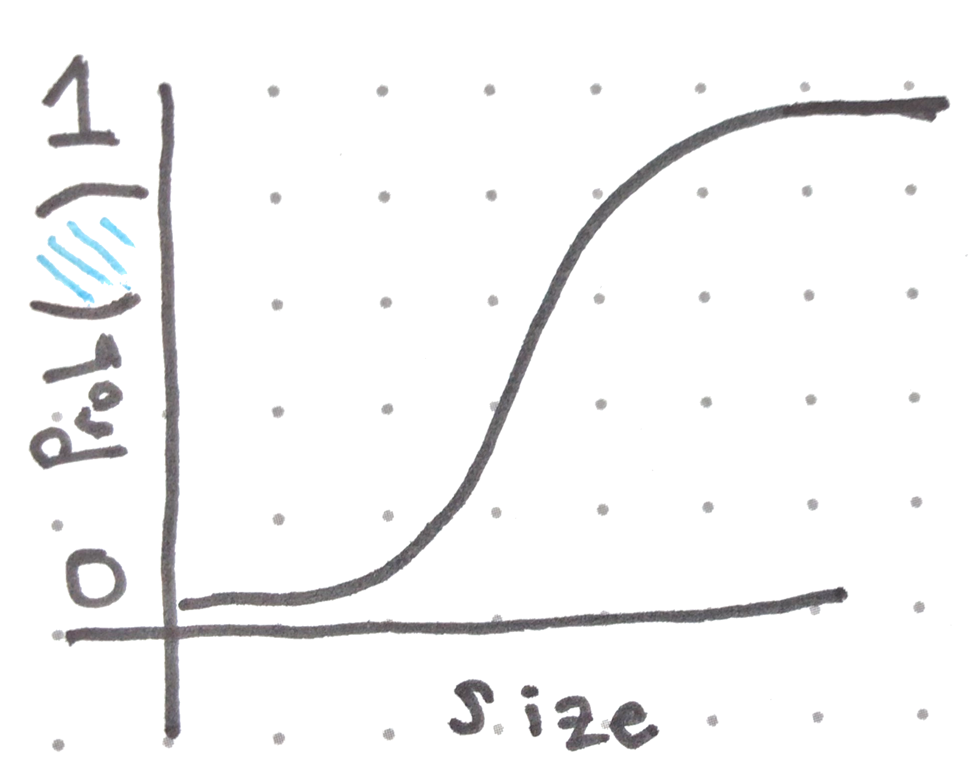
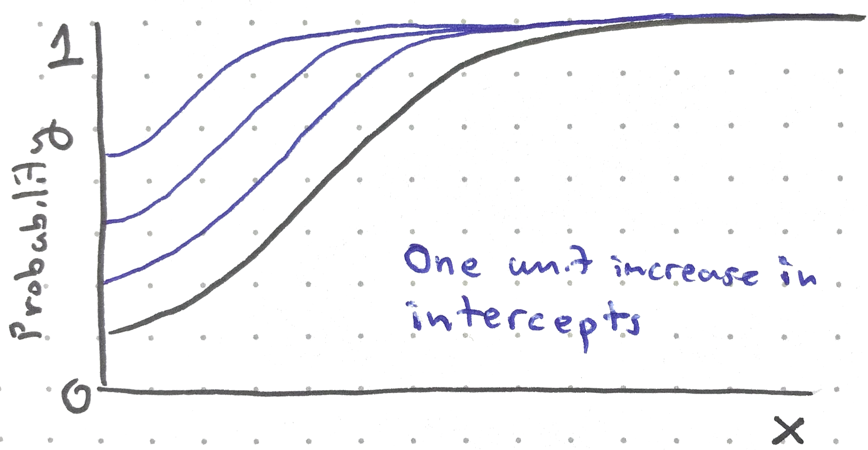
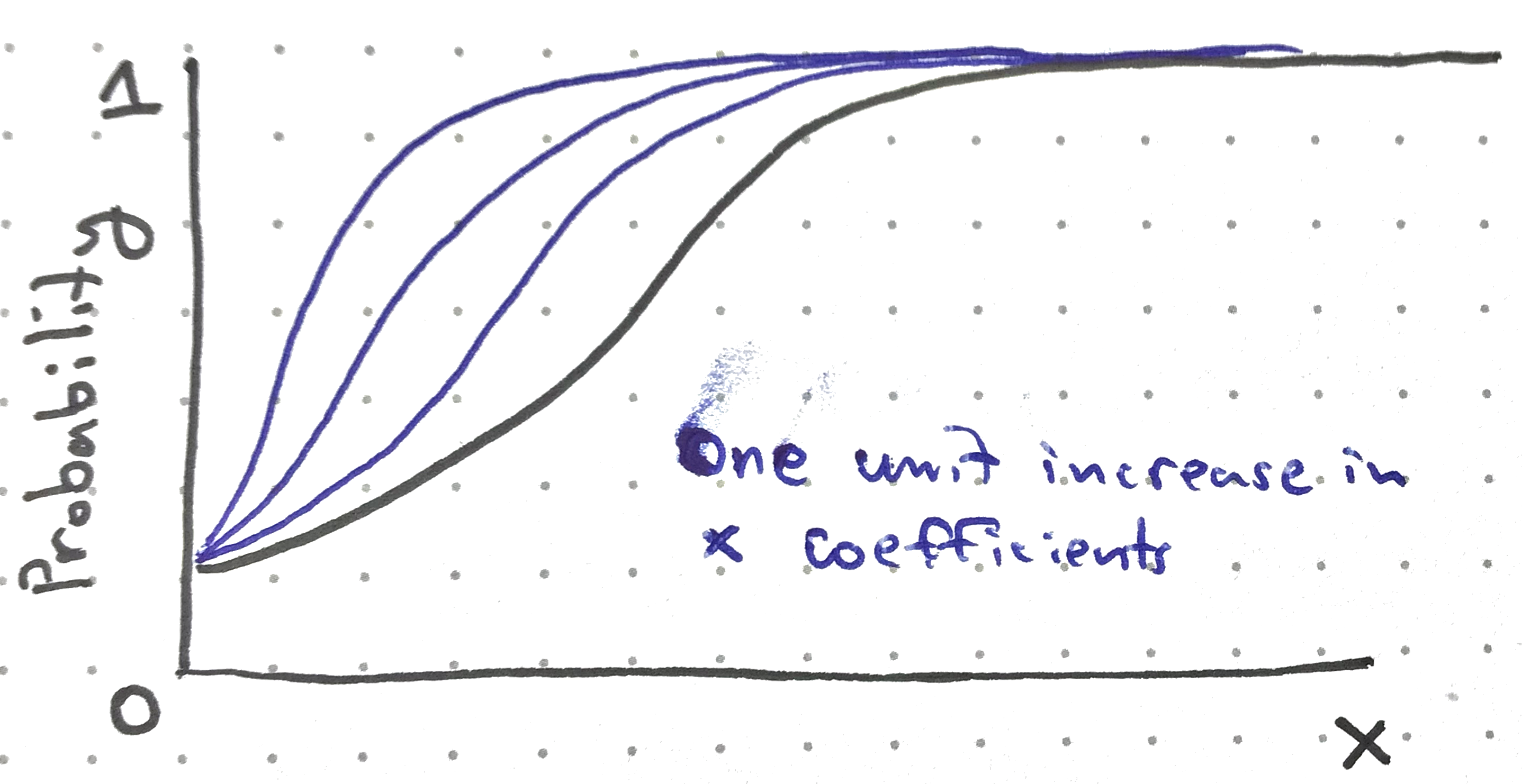
• The intercept parameter controls the height of the curve at 0.
• The slope parameter controls the rate of its increase as a function of \(x\).

Interpreting the fit

• The intercept parameter controls the height of the curve at 0.
• The slope parameter controls the rate of its increase as a function of \(x\).

Interpreting the fit

• x = 0 \(\implies\) plogis(-2.37) ≈ 0.085
• x = 0.5 \(\implies\) plogis(-2.37 + 3.09 * 0.5) ≈ 0.30
• x = 1 \(\implies\) plogis(-2.37 + 3.09 * 1) ≈ 0.67

Poisson Models

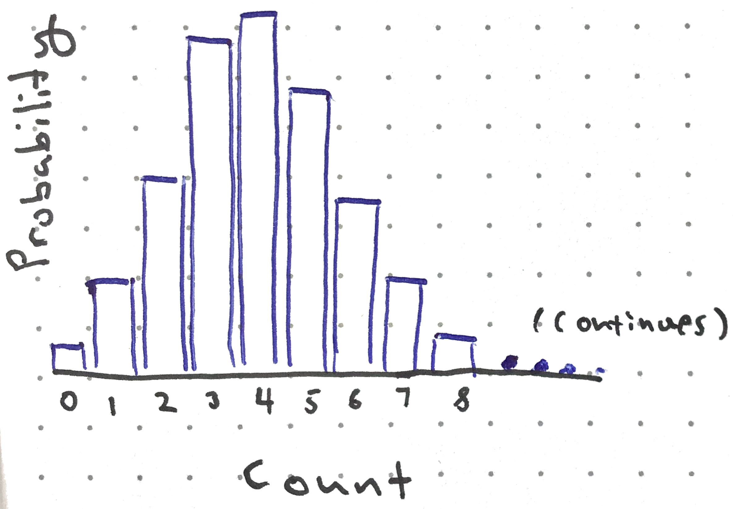
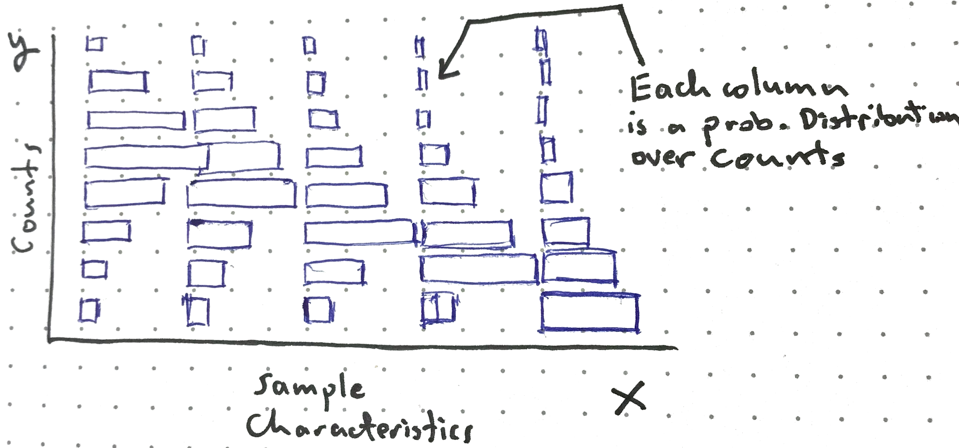
These models apply to count data.

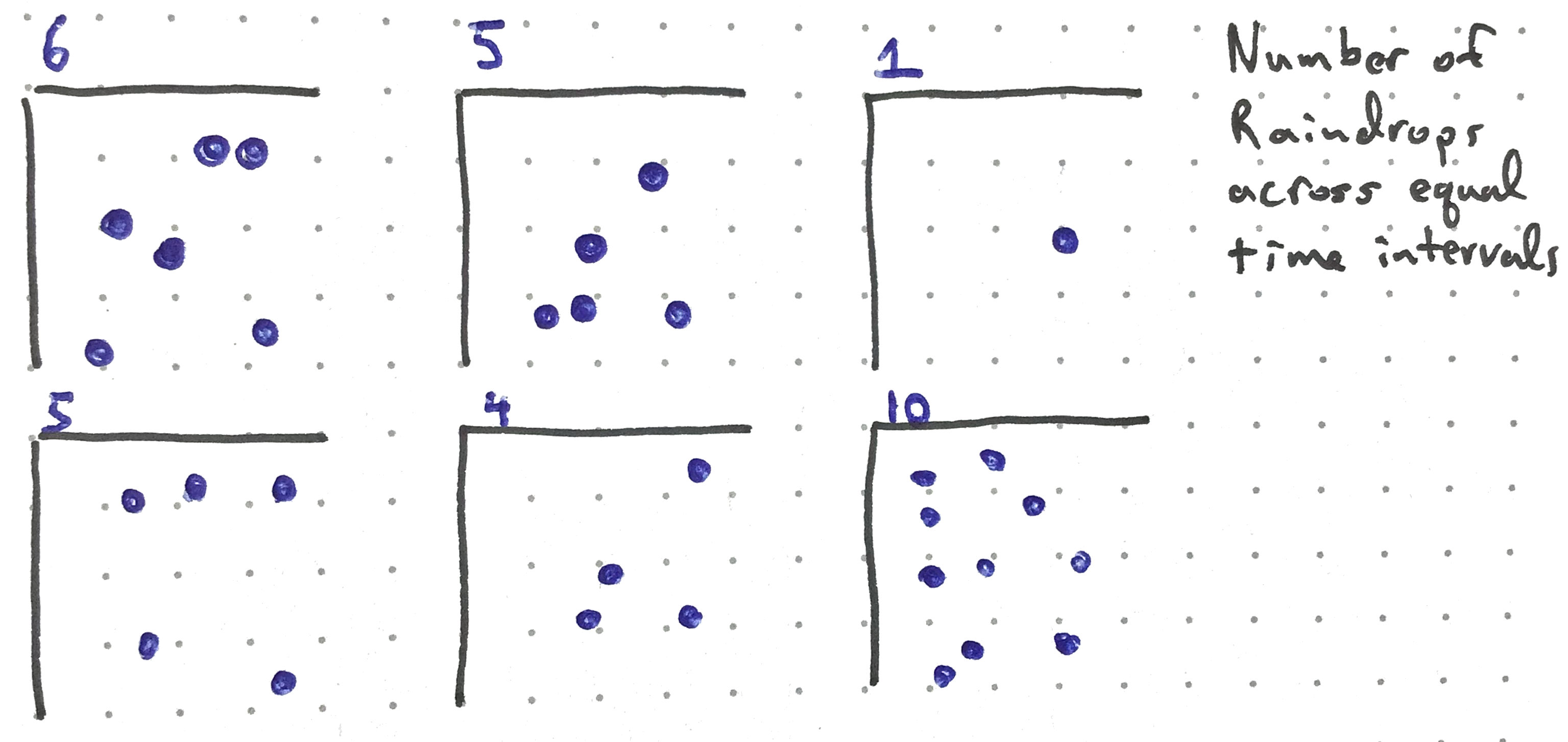
The Poisson arises as the “number of occurrences of an event that happens rarely but has many opportunities to happen” (1). The number of raindrops landing on a small window during a heavy storm would be Poisson distributed.

Poisson Models

These models apply to count data.

The Poisson arises as the “number of occurrences of an event that happens rarely but has many opportunities to happen” (1). The number of raindrops landing on a small window during a heavy storm would be Poisson distributed.

Poisson Models

Counts can depend on sample characteristics. The rain may have been falling harder earlier in the night.

Poisson Models

Many biological counts have this flavor:

• Transcript counts
  • Many transcripts, each with small chance of binding to cDNA
  • The number of transcripts of a gene might depend on drug treatment
• Mutation count along a genome segment
  • Many base pairs with small chance of being mutated
  • The number of mutations depends on selection pressure
• Infection count within a county
  • Many people with small probability of being infected
  • The infection rates decrease further from the epicenter

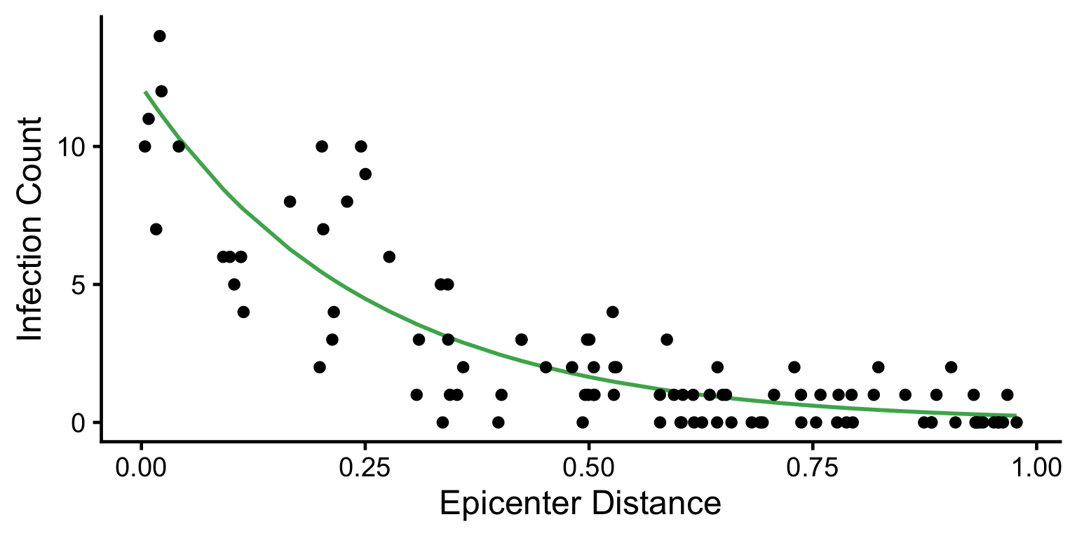
Outbreak counts vs. distance

Let’s fit a model for the infection count example.

Outbreak counts vs. distance

Counts can depend on sample characteristics, like more infections in counties closer to the outbreak epicenter.

Table 2

outbreak |>
    select(sample_id, epicenter_distance, infected)

# A tibble: 100 × 3
   sample_id epicenter_distance infected
   <chr>                  <dbl>    <dbl>
 1 sample_1               0.952        0
 2 sample_2               0.213        3
 3 sample_3               0.498        3
 4 sample_4               0.307        1
 5 sample_5               0.888        1
 6 sample_6               0.605        1
 7 sample_7               0.930        1
 8 sample_8               0.737        0
 9 sample_9               0.399        0
10 sample_10              0.104        5
# ℹ 90 more rows

Fitting the Poisson

fit <- glm(infected ~ epicenter_distance, family = poisson(), data = outbreak)
summary(fit)

Call:
glm(formula = infected ~ epicenter_distance, family = poisson(), 
    data = outbreak)

Coefficients:
                   Estimate Std. Error z value Pr(>|z|)    
(Intercept)         2.41503    0.09458   25.54   <2e-16 ***
epicenter_distance -3.89306    0.27251  -14.29   <2e-16 ***
---
Signif. codes:  0 '***' 0.001 '**' 0.01 '*' 0.05 '.' 0.1 ' ' 1

(Dispersion parameter for poisson family taken to be 1)

    Null deviance: 364.28  on 99  degrees of freedom
Residual deviance: 108.18  on 98  degrees of freedom
AIC: 304.64

Number of Fisher Scoring iterations: 5

The output is on the log scale, so exponentiate before interpreting.

Interpreting the fit

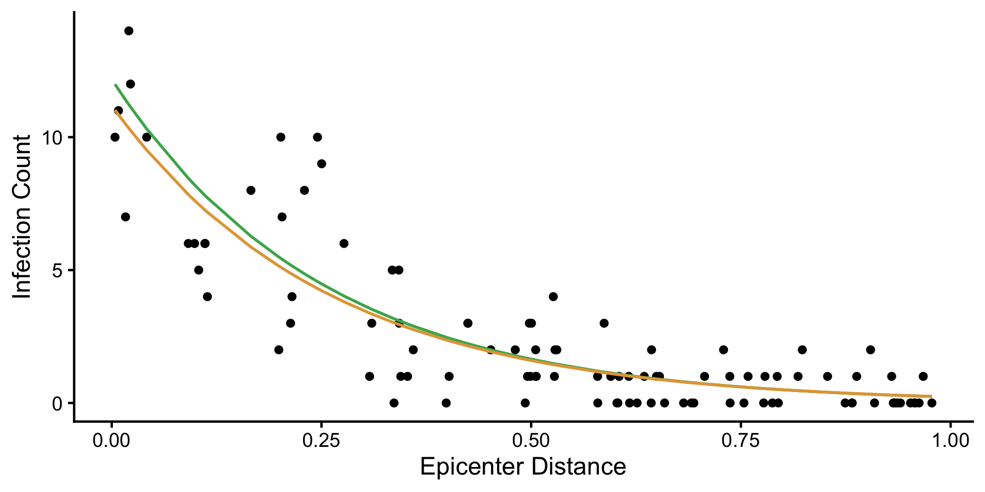
At distance x, the average count is ≈ exp(2.4 - 3.9x)

• x = 0 \(\implies\) exp(2.4) ≈ 11.0
• x = 0.5 \(\implies\) exp(2.4 − 3.9 * 0.5) ≈ 1.6

Call:
glm(formula = infected ~ epicenter_distance, family = poisson(), 
    data = outbreak)

Coefficients:
                   Estimate Std. Error z value Pr(>|z|)    
(Intercept)         2.41503    0.09458   25.54   <2e-16 ***
epicenter_distance -3.89306    0.27251  -14.29   <2e-16 ***
---
Signif. codes:  0 '***' 0.001 '**' 0.01 '*' 0.05 '.' 0.1 ' ' 1

(Dispersion parameter for poisson family taken to be 1)

    Null deviance: 364.28  on 99  degrees of freedom
Residual deviance: 108.18  on 98  degrees of freedom
AIC: 304.64

Number of Fisher Scoring iterations: 5

Interpreting the fit

At distance x, the average count is ≈ exp(2.4 - 3.9x)

• x = 0 \(\implies\) exp(2.4) ≈ 11.0
• x = 0.5 \(\implies\) exp(2.4 − 3.9 * 0.5) ≈ 1.6

Linear Regression Models

Linear regression applies when the response is continuous. For example:

• Temperature
• Antibody titre
• Leaf width

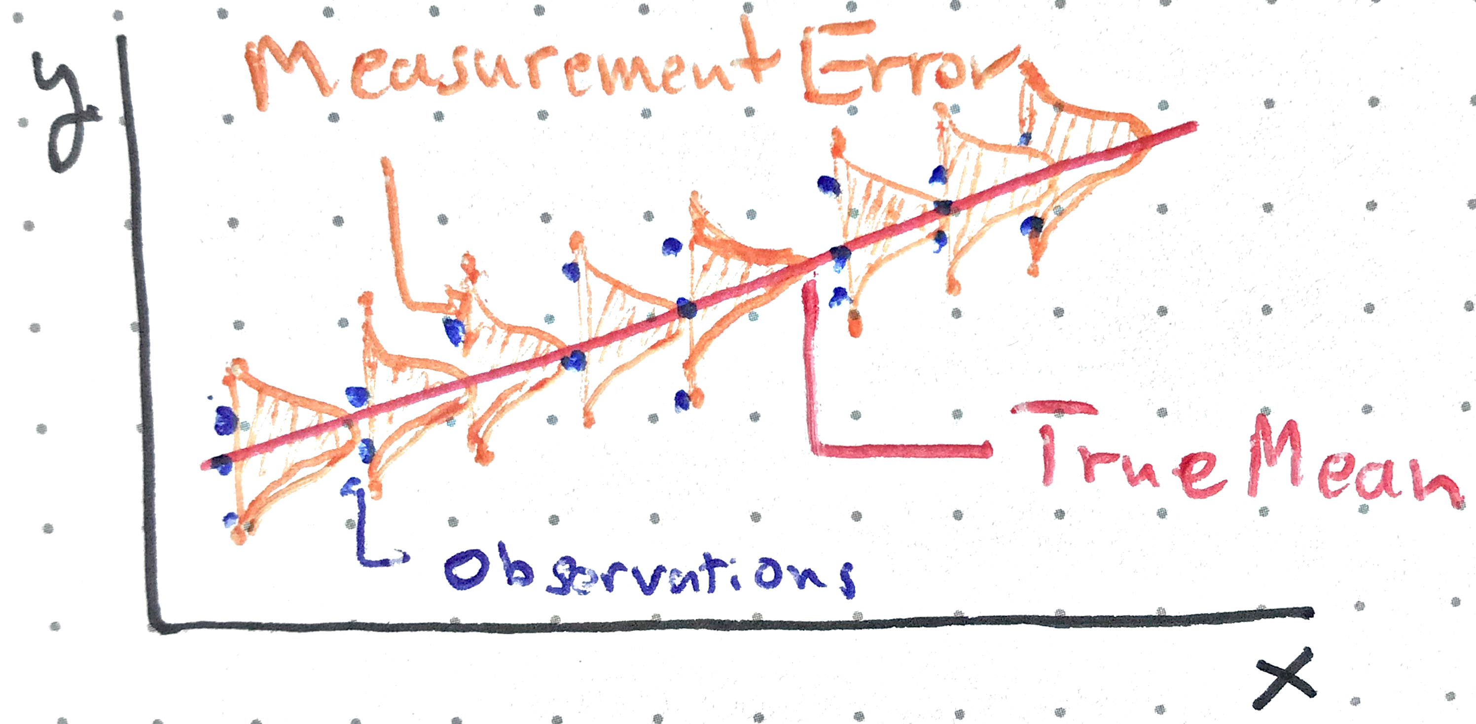
The model assumes random Gaussian error around a mean value that depends on the covariates.

Gaussian Assumption

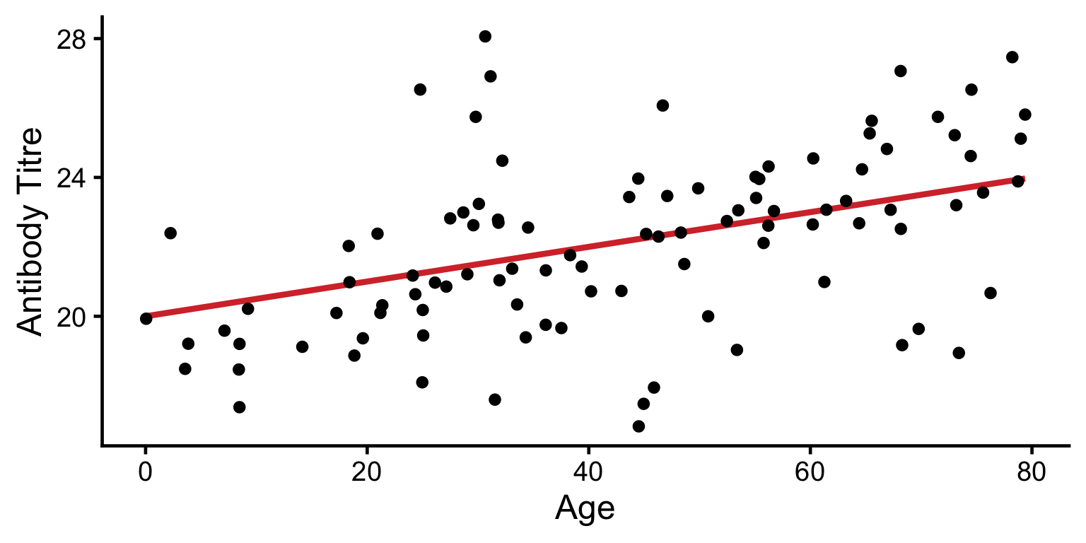
Antibody titre vs age

Fitting with lm

Same inputs as glm, but no family.

fit <- lm(antibody ~ age, data = antibody)
summary(fit)

Call:
lm(formula = antibody ~ age, data = antibody)

Residuals:
   Min     1Q Median     3Q    Max 
-5.345 -1.076 -0.076  1.325  6.698 

Coefficients:
            Estimate Std. Error t value Pr(>|t|)    
(Intercept) 19.57687    0.49545  39.514  < 2e-16 ***
age          0.05834    0.01041   5.606 1.91e-07 ***
---
Signif. codes:  0 '***' 0.001 '**' 0.01 '*' 0.05 '.' 0.1 ' ' 1

Residual standard error: 2.205 on 98 degrees of freedom
Multiple R-squared:  0.2428,    Adjusted R-squared:  0.2351 
F-statistic: 31.42 on 1 and 98 DF,  p-value: 1.911e-07

Interpreting the fit

The estimates are on the same scale as the response, so we can interpret the results directly.

Call:
lm(formula = antibody ~ age, data = antibody)

Residuals:
   Min     1Q Median     3Q    Max 
-5.345 -1.076 -0.076  1.325  6.698 

Coefficients:
            Estimate Std. Error t value Pr(>|t|)    
(Intercept) 19.57687    0.49545  39.514  < 2e-16 ***
age          0.05834    0.01041   5.606 1.91e-07 ***
---
Signif. codes:  0 '***' 0.001 '**' 0.01 '*' 0.05 '.' 0.1 ' ' 1

Residual standard error: 2.205 on 98 degrees of freedom
Multiple R-squared:  0.2428,    Adjusted R-squared:  0.2351 
F-statistic: 31.42 on 1 and 98 DF,  p-value: 1.911e-07

Predicted titre at age x is 19.6 + 0.058x

E.g. at age 10 the prediction is ≈ 19.6 + 0.58 = 20.18

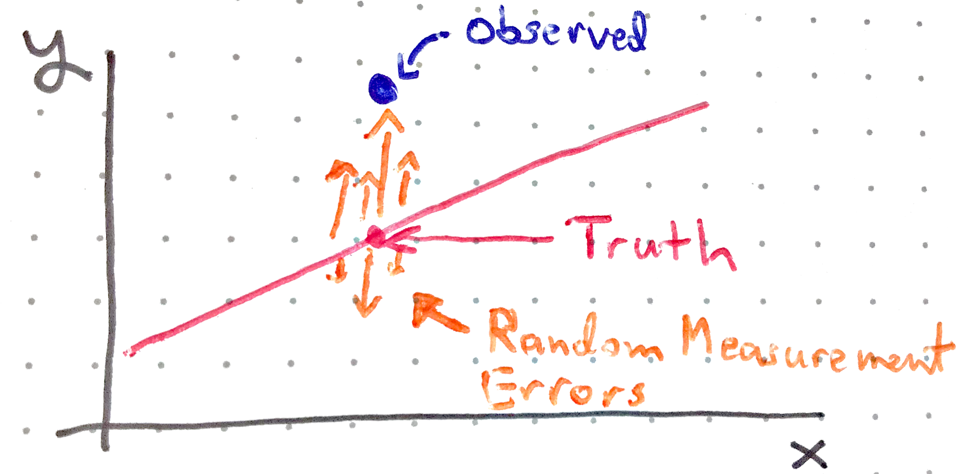
Why Gaussian errors?

The Central Limit Theorem: the average of many small, independent effects tends toward a Gaussian distribution.

We implicitly assume many small, independent factors other than age that perturb the observed antibody measurement.

Discussion

Recommend a model for each of the following questions. What plot would you use to validate your choice? What would be the response and covariate variables?

• We have counts of gene transcripts over time from a bulk RNA-sequencing experiment. Is its expression systematically changing?
• Study participants have been grouped into low and high inflammation groups. We want to see whether abundance of a given microbe-produced metabolite is associated with inflammation group.
• Study participants have been grouped into HIV-free and HIV-positive groups. We want to see whether HIV status is related to proportion of Lactobacillus in the vaginal microbiome.

Variations: Multiple Predictors, Mixed Effects, Interactions

Multiple Predictors

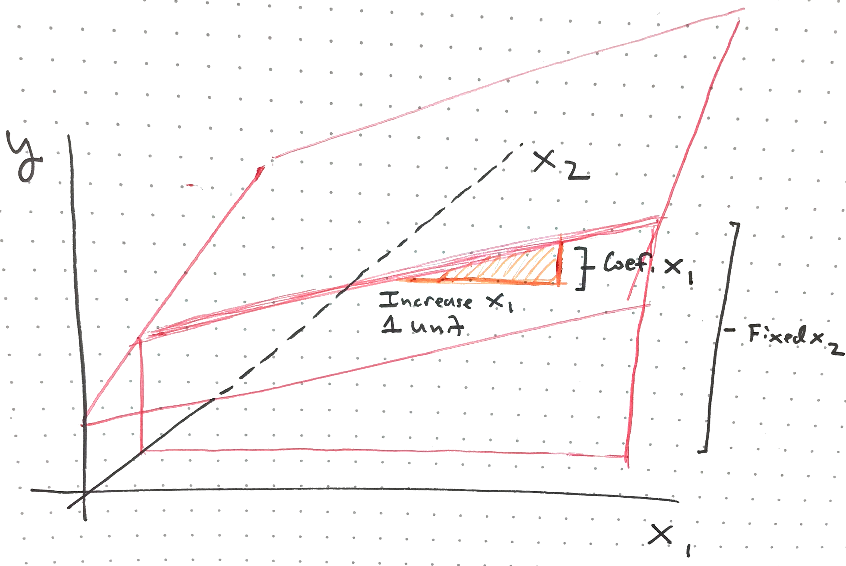
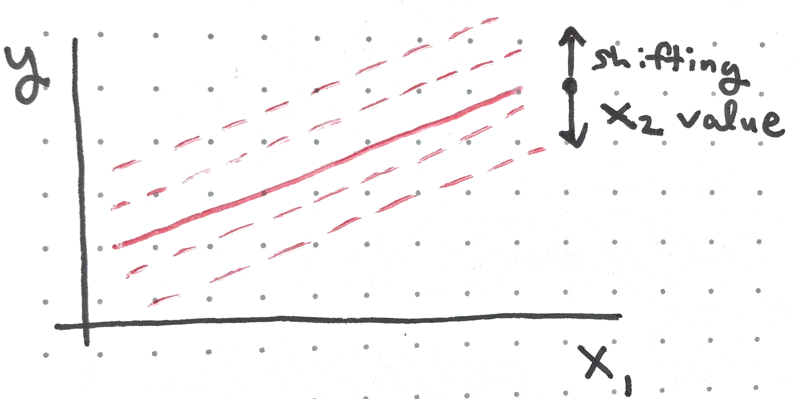
Formulas can have multiple covariates: y ~ x1 + x2

Each estimate is the effect of a variable with all others held fixed.

fit <- lm(antibody ~ age + blood_pressure, data = antibody)
summary(fit)

Call:
lm(formula = antibody ~ age + blood_pressure, data = antibody)

Residuals:
   Min     1Q Median     3Q    Max 
-5.014 -1.044 -0.175  1.288  6.525 

Coefficients:
               Estimate Std. Error t value Pr(>|t|)    
(Intercept)    21.10179    1.10078  19.170  < 2e-16 ***
age             0.05839    0.01033   5.650 1.61e-07 ***
blood_pressure -0.01553    0.01003  -1.549    0.125    
---
Signif. codes:  0 '***' 0.001 '**' 0.01 '*' 0.05 '.' 0.1 ' ' 1

Residual standard error: 2.19 on 97 degrees of freedom
Multiple R-squared:  0.2611,    Adjusted R-squared:  0.2458 
F-statistic: 17.14 on 2 and 97 DF,  p-value: 4.239e-07

Fixing blood pressure, average antibody level increases by 0.058 units per year of age.

Multiple Predictors

Multiple Predictors

Categorical covariates

All models can be used with covariates that are categorical. They are not limited to drawing smooth curves or straight lines.

Categorical covariates

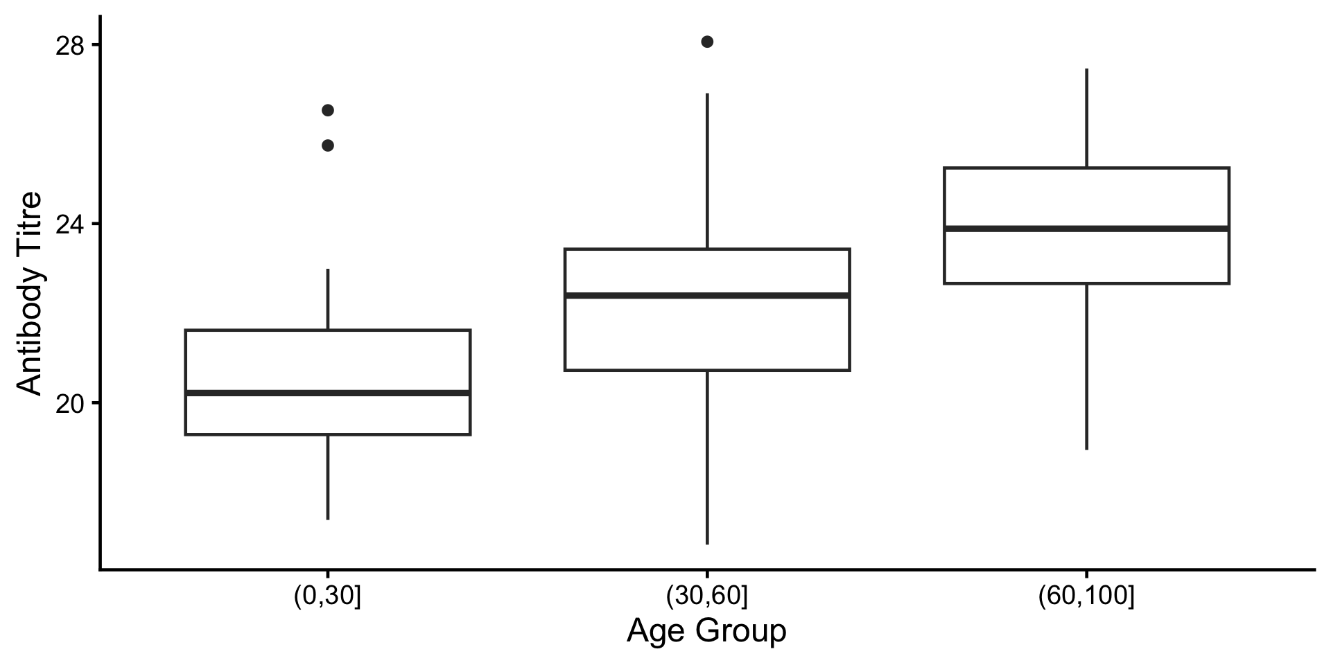
This is a linear regression model fitted to the previous slide’s data, where antibody levels are grouped.

Call:
lm(formula = antibody ~ age_group, data = antibody_grouped)

Residuals:
   Min     1Q Median     3Q    Max 
-5.209 -1.311  0.119  1.429  6.025 

Coefficients:
                  Estimate Std. Error t value Pr(>|t|)    
(Intercept)        20.6901     0.4078  50.737  < 2e-16 ***
age_group(30,60]    1.3476     0.5376   2.507   0.0139 *  
age_group(60,100]   2.9923     0.5977   5.006 2.48e-06 ***
---
Signif. codes:  0 '***' 0.001 '**' 0.01 '*' 0.05 '.' 0.1 ' ' 1

Residual standard error: 2.27 on 97 degrees of freedom
Multiple R-squared:  0.2054,    Adjusted R-squared:  0.189 
F-statistic: 12.54 on 2 and 97 DF,  p-value: 1.436e-05

Mixed effects

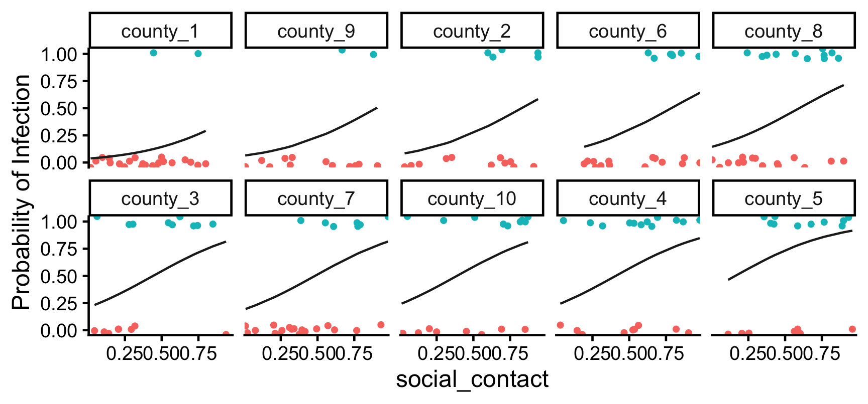
• Baseline effects often vary across contexts.

• In the Bernoulli example, the way infection probability increases with social contact may vary across counties due to unmeasured factors, like population density.

County-varying baselines

Random effects

• We could add county as an ordinary covariate — but with many counties, this becomes unwieldy.
• A better approach is to use a random effect
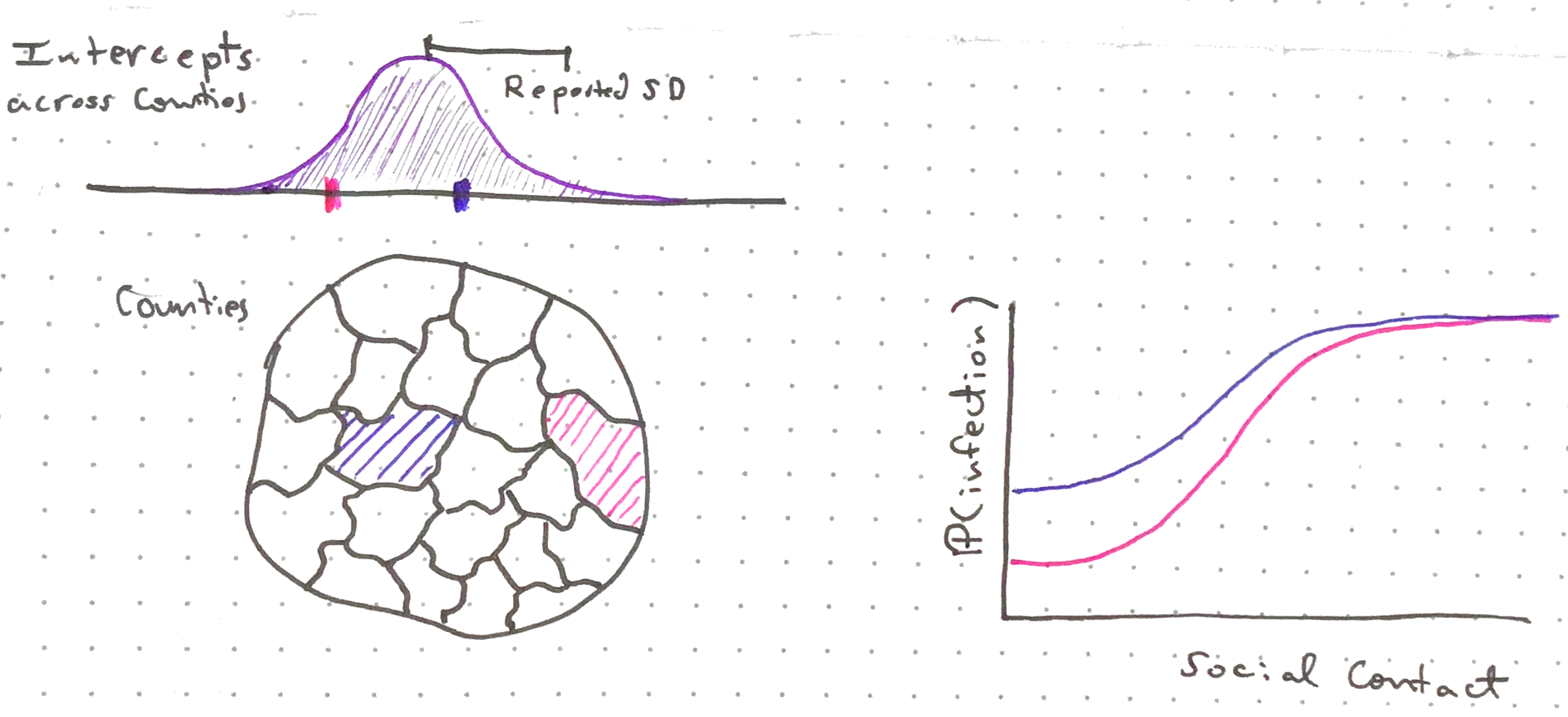
• We imagine county effects as draws from a shared distribution.

Random effects

• We estimate the overall variation across counties, not each one separately.
• This is statistically easier, so it yields higher power.
• Because they include both fixed and random effects, these are called mixed effects models.

Fitting with glmer

Replace glm with glmer and add (1 | county) to the formula.

fit <- glmer(infected ~ social_contact + (1 | county),
             family = binomial(), data = mixed_effect_data)
summary(fit)

Generalized linear mixed model fit by maximum likelihood (Laplace
  Approximation) [glmerMod]
 Family: binomial  ( logit )
Formula: infected ~ social_contact + (1 | county)
   Data: mixed_effect_data

      AIC       BIC    logLik -2*log(L)  df.resid 
    230.8     240.7    -112.4     224.8       197 

Scaled residuals: 
    Min      1Q  Median      3Q     Max 
-2.2664 -0.6116 -0.3655  0.7618  2.5619 

Random effects:
 Groups Name        Variance Std.Dev.
 county (Intercept) 0.5015   0.7082  
Number of obs: 200, groups:  county, 10

Fixed effects:
               Estimate Std. Error z value Pr(>|z|)    
(Intercept)     -2.4680     0.4783  -5.160 2.47e-07 ***
social_contact   3.5811     0.6886   5.201 1.99e-07 ***
---
Signif. codes:  0 '***' 0.001 '**' 0.01 '*' 0.05 '.' 0.1 ' ' 1

Correlation of Fixed Effects:
            (Intr)
socil_cntct -0.808

Interpreting the random effect

The SD says the intercept varies by roughly 0.71 across counties, at any level of social contact. Therefore, even at social contact = 0, the infection probabilities below would both be typical:

plogis(-2.47 - 2 * 0.71)

[1] 0.02003571

plogis(-2.47 + 2 * 0.71)

[1] 0.2592251

Interactions

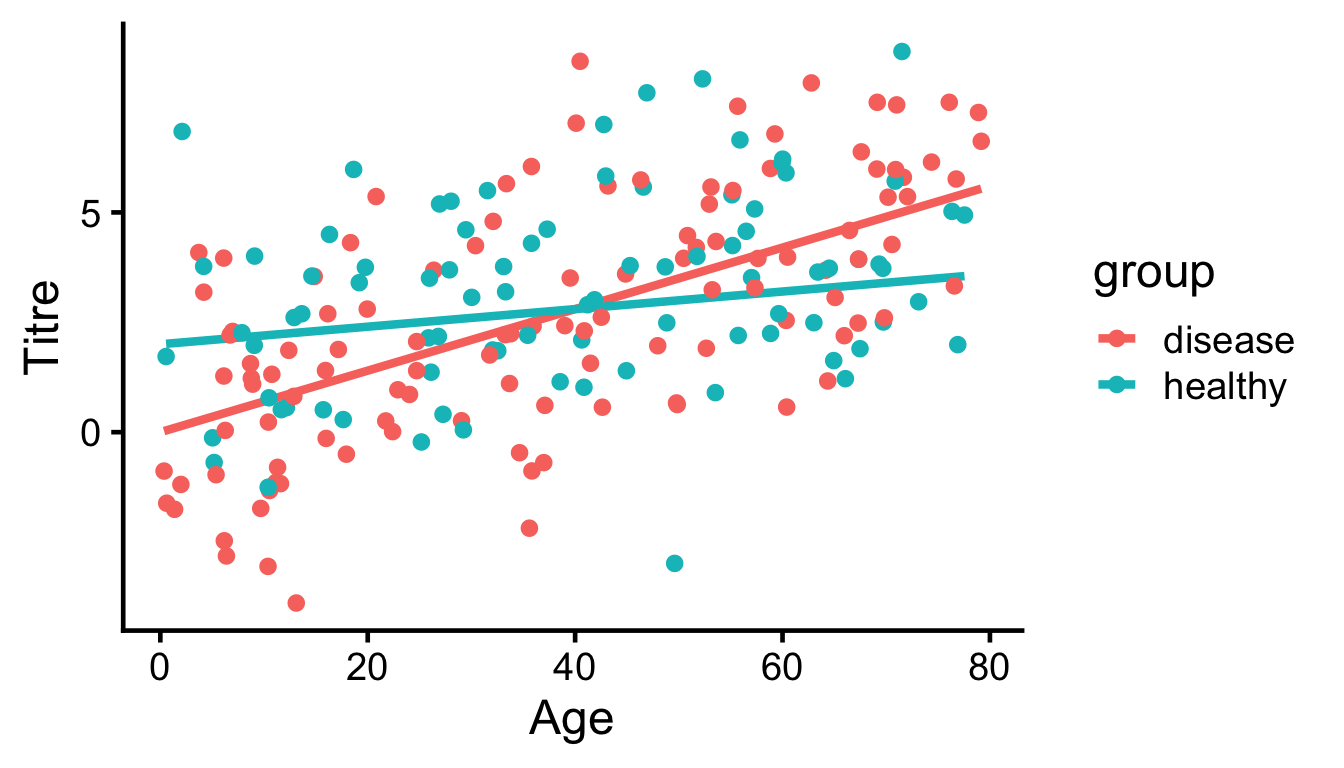
Sometimes the effect of a variable on the response depends on the value of other variables. This is called an interaction.

Interaction syntax

Use y ~ x1 + x1 : x2 — meaning the x1 effect depends on the level of x2.

fit <- lm(antibody ~ age + age : group, data = interaction_data)
summary(fit)

Call:
lm(formula = antibody ~ age + age:group, data = interaction_data)

Residuals:
    Min      1Q  Median      3Q     Max 
-6.4765 -1.6597 -0.0768  1.5193  6.1728 

Coefficients:
                  Estimate Std. Error t value Pr(>|t|)    
(Intercept)       0.543777   0.300945   1.807   0.0723 .  
age               0.061801   0.007332   8.428 7.31e-15 ***
age:grouphealthy -0.002380   0.006885  -0.346   0.7300    
---
Signif. codes:  0 '***' 0.001 '**' 0.01 '*' 0.05 '.' 0.1 ' ' 1

Residual standard error: 2.158 on 197 degrees of freedom
Multiple R-squared:  0.293, Adjusted R-squared:  0.2858 
F-statistic: 40.82 on 2 and 197 DF,  p-value: 1.47e-15

• Healthy group: titre rises by 0.062 per year of age
• Disease group: titre rises by 0.062 - 0.002 per year (sum the two rows)

Variations recap

• Although we introduced these with Bernoulli and linear regression examples, they apply to any of the models we’ve seen.

• They are the key tools we can use when revising a model’s working assumptions to improve its fit.

Discussion

Think through the first three parts of the modeling checklist for a dataset that you are interested in from your own work or study.

1. Biological Question. What real-world questions do you want to answer?

2. Plot the Data. Did you ever plot the data? If so, what patterns did you see? If not, what plots could you make?

3. Working Assumptions. Make a small-world story about your data. What model type, response \(y\), and covariates \(x\) could you use?

Part 3: Case Studies

Case Study: Longitudinal Cytokines

Biological Question

Does treatment with the anti-inflammatory drug change cytokine concentrations post-treatment (week 1), and if so does the effect persist into the long run (week 7)?

Plot the data

There seems to be a strong treatment effect at one week that weakens by week 7. We’ll focus on IL-1a, the cytokine with the fewest measurements below the detection limit.

Working assumptions

• Luminex gives a continuous readout → linear regression
• Many small, unrelated factors perturb the measurement → Gaussian error
• Errors are likely multiplicative, not additive → model log-concentration

A first model

cytokines <- cytokines |> filter(cytokine == "IL-1a")
fit <- lm(log(conc) ~ arm, data = cytokines)
summary(fit)

Call:
lm(formula = log(conc) ~ arm, data = cytokines)

Residuals:
    Min      1Q  Median      3Q     Max 
-2.8298 -0.7570 -0.0689  0.6711  3.7742 

Coefficients:
             Estimate Std. Error t value Pr(>|t|)    
(Intercept)    4.4001     0.1276  34.486  < 2e-16 ***
armtreatment  -1.2410     0.1847  -6.719 5.18e-10 ***
---
Signif. codes:  0 '***' 0.001 '**' 0.01 '*' 0.05 '.' 0.1 ' ' 1

Residual standard error: 1.06 on 130 degrees of freedom
Multiple R-squared:  0.2578,    Adjusted R-squared:  0.2521 
F-statistic: 45.15 on 1 and 130 DF,  p-value: 5.176e-10

The treatment effect is significant, but we should interpret a model only after checking its fidelity.

Check by simulation

The simulate function lets you simulate new response values. By default each simulated output matches the corresponding training sample.

simulate(fit)$sim_1

  [1] 2.9782474 6.0056472 4.6327290 3.7430813 3.5097814 5.1458344 4.5135263
  [8] 5.1387133 4.4975827 4.5481366 6.4344731 2.8556228 4.9953841 2.0500680
 [15] 4.0052839 5.4021195 3.6101001 4.5343215 4.8250682 4.5887460 3.7720848
 [22] 4.5184610 2.6803282 4.6261843 3.4404870 3.3533365 2.4449162 3.5283287
 [29] 3.4626330 2.2391925 2.9518091 1.9920836 2.1450500 4.6969986 6.6768738
 [36] 3.3847478 5.7555652 3.9405248 4.3984729 5.1203345 3.5206530 4.6858492
 [43] 4.7225900 4.0776217 3.8196220 4.3564437 4.2561353 5.0029103 3.9887328
 [50] 3.7775043 3.0674642 3.0946751 2.9118487 4.0622687 5.7886975 5.0469376
 [57] 4.6218549 4.4094212 2.5883835 3.6234321 4.7350077 3.9779685 3.5437505
 [64] 4.1855129 3.2432183 5.0063909 3.9797440 4.6439749 4.5911723 4.0344294
 [71] 5.5723322 4.9410032 1.5954450 2.1826993 4.5523856 4.2886943 2.2728754
 [78] 4.2109297 3.6347512 4.4969185 2.1934358 4.2587041 3.5371852 1.3782517
 [85] 3.3798805 2.9604233 4.0369129 5.7988303 3.8604942 3.1895635 4.7362505
 [92] 4.1814273 5.0781209 3.2112666 3.1003526 4.8286527 3.4191788 3.0124659
 [99] 3.3845371 4.0511941 5.2224927 5.1819689 5.1883101 4.3829128 4.5848620
[106] 5.1636166 4.2656986 5.5124452 2.5322445 2.2851774 3.7349694 4.1399135
[113] 2.8860256 4.4688755 3.9835402 3.2328957 2.3437614 2.0541907 3.2562084
[120] 0.2153196 3.3757924 4.6326766 4.9712758 4.0738577 6.0081757 4.2066597
[127] 3.8932396 4.4853314 3.4849389 4.0478774 2.6657909 4.7393394

Check by simulation

The simulate_cytokines helper function runs simulate and reshapes the data for plotting.

sim_data <- simulate_cytokine(fit)
plot_cytokine(sim_data)

What went wrong?

• ✅ Overall concentrations are in the correct range
• ✅ Control group has larger concentrations than treatment
• ❌ In the real data, most blue curves decrease at week 1
• ❌ In the simulation, about half the curves increase

Revising the model

• We gave the model no temporal information. We could fix this with the formula: log(conc) ~ arm + time_point.

  • This data story isn’t reasonable either
  • We don’t expect IL-1a concentration to change just because the clock reads week 1 or 7.

We want the treatment effect itself to depend on the week, a type of interaction: log(conc) ~ arm + arm : time_point.

Fitted interaction model

fit <- lm(log(conc) ~ arm + arm : time_point, data = cytokines)
summary(fit)

Call:
lm(formula = log(conc) ~ arm + arm:time_point, data = cytokines)

Residuals:
     Min       1Q   Median       3Q      Max 
-2.36776 -0.57246  0.00535  0.47567  2.64101 

Coefficients:
                              Estimate Std. Error t value Pr(>|t|)    
(Intercept)                     4.6636     0.1718  27.147  < 2e-16 ***
armtreatment                   -0.2855     0.2487  -1.148   0.2531    
armplacebo:time_pointweek_1    -0.4784     0.2429  -1.969   0.0511 .  
armtreatment:time_pointweek_1  -2.3398     0.2543  -9.203 9.50e-16 ***
armplacebo:time_pointweek_7    -0.3121     0.2429  -1.285   0.2013    
armtreatment:time_pointweek_7  -1.3173     0.2543  -5.181 8.51e-07 ***
---
Signif. codes:  0 '***' 0.001 '**' 0.01 '*' 0.05 '.' 0.1 ' ' 1

Residual standard error: 0.8239 on 126 degrees of freedom
Multiple R-squared:  0.5653,    Adjusted R-squared:  0.5481 
F-statistic: 32.77 on 5 and 126 DF,  p-value: < 2.2e-16

Interpreting the coefficients

Expected log-concentrations:

• Placebo at baseline: 4.66
• Treatment at baseline: 4.66 − 0.29
• Placebo at week 1: 4.66 − 0.48
• Treatment at week 1: 4.66 − 2.34
• …

The large negative coefficient for armtreatment:time_pointweek_1 captures our earlier observation that the treatment effect is strongest at week 1.

Simulate updated model

Mixed-effects version

The model treats each sample as independent, but measurements from the same participant are dependent.

• Dependence reduces the effective sample size.
• We can add a participant-level random effect to introduce dependence.

fit <- lmer(log(conc) ~ arm + arm : time_point + (1 | pid), data = cytokines)

Simulate updated model

Model results

summary(fit)

Linear mixed model fit by REML. t-tests use Satterthwaite's method [
lmerModLmerTest]
Formula: log(conc) ~ arm + arm:time_point + (1 | pid)
   Data: cytokines

REML criterion at convergence: 327.2

Scaled residuals: 
    Min      1Q  Median      3Q     Max 
-2.8408 -0.6889 -0.0017  0.5540  3.1092 

Random effects:
 Groups   Name        Variance Std.Dev.
 pid      (Intercept) 0.02198  0.1483  
 Residual             0.65679  0.8104  
Number of obs: 132, groups:  pid, 44

Fixed effects:
                              Estimate Std. Error       df t value Pr(>|t|)    
(Intercept)                     4.6636     0.1718 125.7363  27.147  < 2e-16 ***
armtreatment                   -0.2855     0.2487 125.7363  -1.148   0.2531    
armplacebo:time_pointweek_1    -0.4784     0.2390  83.9999  -2.002   0.0485 *  
armtreatment:time_pointweek_1  -2.3398     0.2501  83.9999  -9.355 1.14e-14 ***
armplacebo:time_pointweek_7    -0.3121     0.2390  83.9999  -1.306   0.1952    
armtreatment:time_pointweek_7  -1.3173     0.2501  83.9999  -5.267 1.05e-06 ***
---
Signif. codes:  0 '***' 0.001 '**' 0.01 '*' 0.05 '.' 0.1 ' ' 1

Correlation of Fixed Effects:
            (Intr) armtrt armp:__1 armt:__1 armp:__7
armtreatmnt -0.691                                  
armplcb:__1 -0.696  0.481                           
armtrtm:__1  0.000 -0.503  0.000                    
armplcb:__7 -0.696  0.481  0.500    0.000           
armtrtm:__7  0.000 -0.503  0.000    0.500    0.000  

Interpretation

• Visually, the model doesn’t seem much better.
• Participant variation (SD 0.15) is small vs. measurement error (0.81).
• But it’s the safer model in practice. By accounting for within-participant dependence, we’re being honest about the effective sample size.

Wrapping Up

What we did today

1. Models as data stories — small world vs. large world.
2. A modeling checklist to guide our work: question → plot → assumptions → checks → revise.
3. A review of modeling ingredients: Bernoulli, Poisson, Linear.
4. Variations for complex data: multiple predictors, mixed effects, interactions.
5. Case study illustrating the checklist

Exercise 1

Open notebooks/05-modeling.qmd in your Codespace.

The modes flip: whoever was agentic in Exercise 1 is manual now, and vice versa.

Exercise 2

Open notebooks/05-modeling.qmd in your Codespace.

The modes flip: whoever was agentic in Exercise 1 is manual now, and vice versa.

1.

Wikipedia. Poisson distribution — Wikipedia, the free encyclopedia [Internet]. 2026. Available from: http://en.wikipedia.org/w/index.php?title=Poisson%20distribution&oldid=1355788475